Probabilistic derivation of Black-Scholes using martingales, change of measure, and Girsanov's theorem. Discounted asset prices, self-financing replication, no-arbitrage, and the fundamental asset pricing formula connect risk-neutral valuation to Monte Carlo intuition.
How are you doing today? Module 3 is pretty steep. We're not exactly going to change the trend tonight. We'll change gear a little bit to something more thoughtful and meditative on Thursday, but tonight we're going to continue with all the things you like about Module 3, which is Black-ScholesBlack-Scholes Black-Scholes is the standard continuous-time framework for pricing options and related derivatives., option pricingOption pricing Option pricing is the process of determining a fair value for an option from its payoff and model assumptions.. We're going to do it all over again, using different tools.
There are several good reasons to do so. The first one is that there are actually many different ways to get to Black-ScholesBlack-Scholes Black-Scholes is the standard continuous-time framework for pricing options and related derivatives.. As long as your assumptions are coherent and consistent, you have many different approaches that will give you the Black-Scholes equationBlack-Scholes equation The Black-Scholes equation is the PDE that the option price satisfies in the standard Black-Scholes model., and each one carries slightly different insights. That's one of the beautiful things about math: there are always several approaches that you can take to derive the same results.
We're going to start exploiting that tonight, because we'll see the second most important way of getting to Black-Scholes, which is using probability theory. What you've learned so far is Black-Scholes using PDEsPDE / partial differential equation PDE stands for partial differential equation.. We'll also see on Thursday that you can get Black-Scholes from the binomial modelBinomial model The binomial model is a discrete-time model where an asset price moves up or down by fixed factors over successive steps., and that's something we use to draw links between the various ways that we've done Black-Scholes.
In fact, years ago, probably 14 years ago, the ever-young Paul Wilmott and the not-so-ever-young me did a lecture together where we reviewed 10 ways of deriving Black-Scholes. There are plenty of ways, and since then Paul has still added a few more to the list. That's a lecture that's on the portal, and given that it's 15 years old, it's probably one of the silent movies in black and white. Okay, now I'm exaggerating a bit.
Today we are going to look at probabilistic methods, and the key term is actually going to be martingalesMartingale A martingale is a stochastic process with no predictable drift under the relevant information set.. When we talk about martingales, we are actually thinking about three different concepts that you've probably already encountered in the CQF, and if you didn't, we're going to talk a bit about that tonight. That's actually at the heart of the method.
The first one is that you know that a martingaleMartingale A martingale is a stochastic process with no predictable drift under the relevant information set. is a stochastic processStochastic process A stochastic process is a family of random variables indexed by time. that has a very specific property. First, your stochastic process M_t needs to be integrable. We need to be able to compute its expectationExpectation The average value of a random variable under a probability distribution., so it needs to satisfy the property that the expectation of the absolute value of this process M_t needs to be finite; otherwise, we can't talk about expectation. That's the integrability condition.
So a martingale M_t is a stochastic processStochastic process A stochastic process is a family of random variables indexed by time. that is integrable and has a very unique characteristic: if you take two time periods, today, let's callCall option / call A call option is a derivative that gives the right, but not the obligation, to buy an asset at a fixed strike price. that time t, and then later, let's call that time T, and you observe your process, your martingale, up to time t, so you have access to the filtration F_tFiltration A time-indexed family of information sets describing what is known at each moment., then your best guess for where your martingale is going to be at time T is actually just the value at time t. This is the best guess given the information that you've got so far.
So a martingale is pure noise. That doesn't mean that M_T will be equal to M_t, but on average the expected valueExpectation The average value of a random variable under a probability distribution. of M_T, given information up to time t, is going to be equal to the last known value, which is M_t. Martingales are very convenient processes because they are pure noise. Everything else that can happen is according to a probability distributionProbability distribution A probability distribution describes how probability is assigned across possible outcomes of a random variable., and the mean of this probability distribution is centered at the last known value.
This is why tonight, by using martingales, we have a very heavily probabilistic approach. We're going to use these properties of randomness. The second idea that we're going to see, still connected to martingales, is a very special martingale called an exponential martingaleExponential martingale An exponential martingale is a special martingale formed by exponentiating a stochastic process in a way that preserves the martingale property.. As the name indicates, it's both an exponential and a martingale, hence the term exponential martingale.
One of the nice things about mathematics is that when you have a term that sounds a bit confusing, you say it slowly enough three times, and by the third time you should know what it means, because what we callCall option / call A call option is a derivative that gives the right, but not the obligation, to buy an asset at a fixed strike price. things is actually what they do. It's an exponential process and it's a martingale. How should we call it? Fluffy? No, that doesn't work. Exponential martingaleExponential martingale An exponential martingale is a special martingale formed by exponentiating a stochastic process in a way that preserves the martingale property..
Exponential martingales are a special type of martingale, and these exponential martingales are used for something that's called a change of measureChange of measure A change of measure is a transformation that replaces one probability measure with another, usually by reweighting probabilities. from a probability measure PPhysical measure P / measure P Physical measure P is the real-world probability measure used to model observed asset behavior., the real-world measure, to another one that's called Q. A lot of things are said about probability measures. We're going to illustrate that quite informally as a change of world, but really what it is is very close to a change of variable, except that instead of a change of variable, we change the definition of the Brownian motionBrownian motion Brownian motion is a continuous-time stochastic process with independent, normally distributed increments..
However, it's really just a computational trick. So it's nice to be able to describe the Q world as risk-neutralQ / risk-neutral Q is the risk-neutral measure used in pricing and hedging calculations., or planet finance, and look at its properties, but bottom line is change of measureChange of measure A change of measure is a transformation that replaces one probability measure with another, usually by reweighting probabilities. has nothing arcane or voodoo to it. It's basically a computational trick that we use in order to convert a difficult problem into an easier one, and we're going to use this change of measure twice tonight. So this lecture is very much anchored in probability and in the concept of martingale.
One of the nice things about what we're going to do today is that it gives you some new insight that you did not have with the PDEPDE / partial differential equation PDE stands for partial differential equation.. The PDE has many advantages. It's an invaluable way of getting to Black-Scholes, especially because it's going to help you do all of the local hedgingLocal hedging Local hedging is hedging designed to offset risk over a small time step or in a local neighborhood of the model.. That's what you use the GreeksGreeks Greeks are derivatives or sensitivity measures used to describe how an option price responds to changes in inputs. for: to know that for a small change of price, you can hedge your optionOption A financial contract whose value depends on an underlying asset and may give the holder the right to exercise it. by buying deltaDelta Delta is a sensitivity measure, usually the derivative of an option price with respect to the underlying asset price. shares. For a small change in price, if you want to be more accurate, you combine delta and gamma, etc.
Here we're going to look at the probabilities embedded in Black-Scholes, and in particular this approach is going to be useful to answer one of the standard interview questions. One of the best interview questions, an absolute classic, if you want to check how much someone understands about Black-Scholes, is to ask them this question: write the Black-Scholes formulaBlack-Scholes formula The Black-Scholes formula is the closed-form expression for the price of a standard European option in the Black-Scholes model..
Okay, that's not a question. The question comes next. The question is: now that you've written the Black-Scholes formulaBlack-Scholes formula The Black-Scholes formula is the closed-form expression for the price of a standard European option in the Black-Scholes model., could you show me, or give me, the real-world probability of exercise? What is the probability of exercise of the optionOption A financial contract whose value depends on an underlying asset and may give the holder the right to exercise it. in the real world? Just by asking this question, you can see whether someone understands what the formula is about and what it's telling you from a probability perspective. We'll answer that question by the end of this lecture.
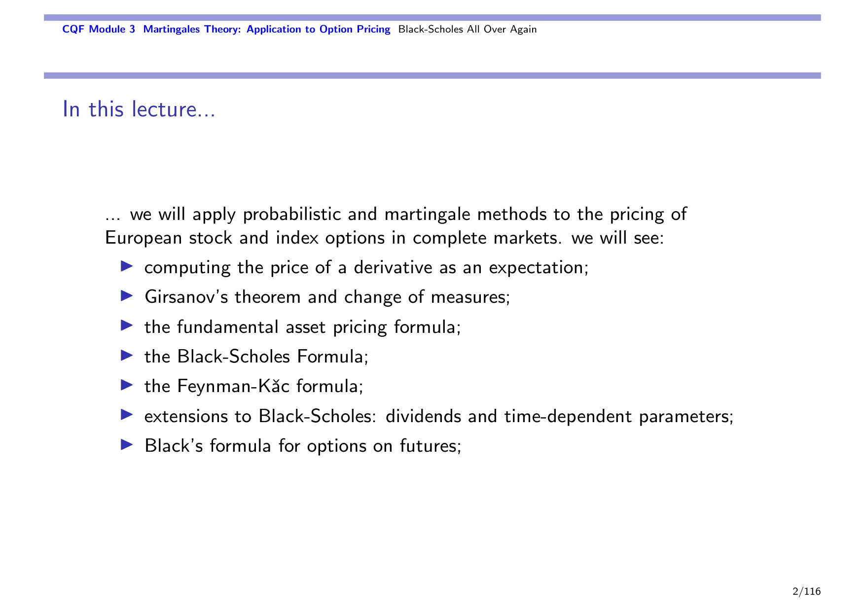
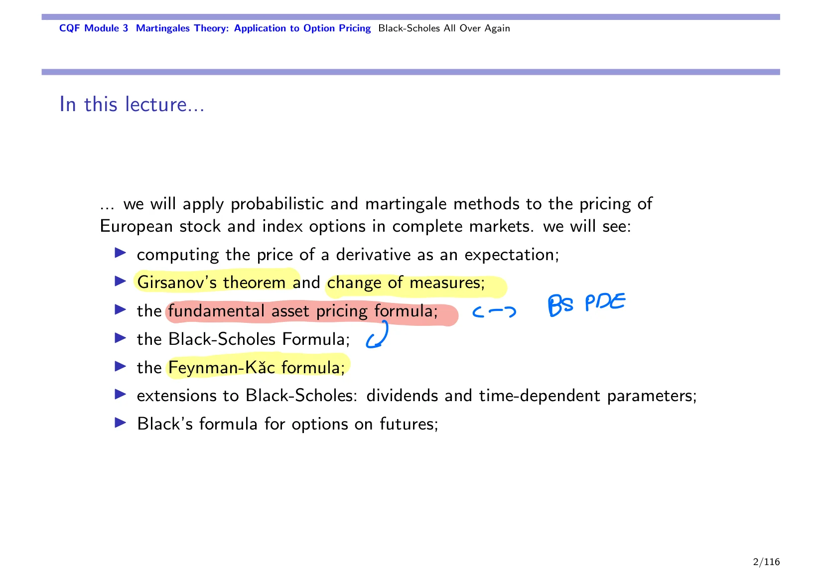
So today we're going to do quite a few things. Well, you know me by now.
Just by asking this question, you can see whether someone understands what the formula is about and what it's telling you from a probability perspective. We will answer that question by the end of this lecture. Today we're going to do quite a few things. We are going to look at how to compute the price of a derivative as an expectationDerivative prices The values assigned to derivative contracts, often computed as an expected discounted payoff..
We are also going to look at something called Girsanov's theoremGirsanov / Girsanov's theorem Girsanov's theorem gives the rule for how stochastic dynamics change under a change of measure.. Girsanov's theorem is the theorem that we use in order to perform these famous changes of measure, which is extremely helpful. We use that very frequently in quantitative finance, precisely with the goal of making a difficult problem easier.
So it's an extremely useful result, which ranks among the top three results in probability and stochastic processes. The first one is, of course, ItôItô Itô refers to the stochastic-calculus framework used to differentiate and integrate random processes., because you are going to use Itô everywhere and all the time. Then the other two results that are trying to jostle for the second spot are actually Girsanov's theoremGirsanov / Girsanov's theorem Girsanov's theorem gives the rule for how stochastic dynamics change under a change of measure. for the change of measure, and something that we discuss on Thursday when we start our next class, which is the Feynman-Kac formulaFeynman-Kac formula A formula connecting solutions of some PDEs with expected values of stochastic processes., which establishes a link between expectations and PDEs.
So Girsanov's theorem and change of measure are at the heart of what we do. We'll use that to develop, or to derive, something that we call the fundamental asset pricing formulaFundamental asset pricing formula The fundamental asset pricing formula prices an asset by taking the discounted expectation of its future payoff under the appropriate measure.. By Thursday night, you will be convinced, I hope, that it is fundamental. By tonight, you will know that it's an asset pricing formula.
The fundamental asset pricing formulaFundamental asset pricing formula The fundamental asset pricing formula prices an asset by taking the discounted expectation of its future payoff under the appropriate measure. in probability plays the same role as the Black-Scholes PDEBlack-Scholes equation The Black-Scholes equation is the PDE that the option price satisfies in the standard Black-Scholes model. in PDEs. By the time we solve this fundamental asset pricing formula, we will get to the Black-Scholes formula.
Now, why do we really need to combine two approaches? One of the reasons is linked to the way our stochastic differential equationSDE / stochastic differential equation SDE stands for stochastic differential equation.s are structured. If you just take a stochastic process, V_t, its dynamics can be expressed as a stochastic differential equation: dV_t is equal to some function f of time and V_t, dt, plus some function g of time and V_t, multiplied by your usual Brownian motionBrownian motion Brownian motion is a continuous-time stochastic process with independent, normally distributed increments.. Then you need an initial condition, so let's set V_0 for some arbitrary value V. Actually, this arbitrary value could be random; it still works.
Now, if you look at this SDESDE / stochastic differential equation SDE stands for stochastic differential equation., you will realize that it really has two parts to it. Set g to zero, then you get dV_t = f(t, V_t) dt, and this is just a good old ordinary differential equationODE / ordinary differential equation ODE stands for ordinary differential equation., purely deterministic, the stuff that we've learned how to work with for the past 200, 250 years, maybe 300 years. Now, if you set f, the driftDrift The deterministic or average directional part of a stochastic process., to zero, then dV_t is just a pure diffusionDiffusion The stochastic part of a continuous-time model that captures random fluctuations. term. It's an ItôItô Itô refers to the stochastic-calculus framework used to differentiate and integrate random processes. diffusion, or in this case even a martingale. So it's pure noise. It's purely random.
When we consider again our stochastic differential equation, we see much better that this is really a wonderful little creature, but it's also a mathematical chimera. It's an equation, or dynamics, made up of parts of other dynamics. It's an ODEODE / ordinary differential equation ODE stands for ordinary differential equation. plus something random. What's more is that these things behave differently.
This term, the driftDrift The deterministic or average directional part of a stochastic process., is deterministic. It scales with dt, so it's of the order of dt, and it tends to dominate when your time horizon is greater than one unit, so for us, one year. But g(t, V_t) dX_t, this is the diffusionDiffusion The stochastic part of a continuous-time model that captures random fluctuations.. It's stochastic, which is really random in time, and scales with the square root of dt, so it doesn't even scale the same way. It dominates over short horizons when your time horizon is less than one unit.
So we really have two different components inside our stochastic differential equation, inside our stochastic dynamics. The point here is that if you want to solve something as complicated as an option price problemOption price problem The task of determining a fair price for an option from its payoff and the market model., it's going to be very hard to keep these two terms happy at the same time. So that has led us to two essential methods.
Method one: turn off the diffusion. This way, you can go back to PDEs. And that's exactly what you've done in Black-Scholes via PDEs. What you've done is create this hedged portfolioHedged portfolio A hedged portfolio is a portfolio arranged so that its value is less sensitive to market risk., because this portfolio is hedged, then the risk goes away. Therefore, this portfolio has a diffusion that's zero. Then you bring in the argument that you want to prevent arbitrageArbitrage Arbitrage is a trading strategy that yields a sure profit without requiring an initial investment or exposing the trader to risk.. This portfolio needs to return the risk-free rater / risk-free rate r is the risk-free rate used as the baseline interest rate in the model., and that gives you your PDE.
What you've done is essentially turn off, through an economic argument, the diffusion. So you went back to the world of ODEs and PDEs, the world of differential equations. The method that we're going to see tonight is: turn off the drift. Then you are in the world of probabilities, or more exactly, in the world of noise. You're in the world of martingales, which are actually easy to deal with by themselves. So that's what we're going to do.
These two methods, of course, method one and method two, are strictly equivalent. However, if we think about the path that they take to reach the Black-Scholes formula, method one, in green, is going to start very nice and easy, slow, slow, up until you get to your first intermediate result, the Black-Scholes PDE.
After that, of course, you've got to solve the PDE. You've got to change your Black-Scholes PDE back into the heat equationHeat equation The heat equation is a partial differential equation describing diffusion or smoothing over time.. Then you solve the heat equation. Then you've got to reverse all of your transformations to finally get to the Black-Scholes formula. So that's essentially how the difficulty evolves in time up until you get to the Black-Scholes formula. The nice thing about this approach is that immediately you get the Black-Scholes PDE.
What we're going to do tonight is a little bit different, because the difficulty is mostly stacked at the start. We are going to have to be a bit more formal. We are going to have to play a little bit with stochastic processes in order to get to the fundamental asset pricing formula. But after that, once we've got that, you could solve this fundamental asset pricing formula using the tools that you already knew before you got into the CQF.
It's just straight integration on your payoff functionPayoff The payoff is the amount received from a contract or strategy, usually evaluated at maturity., so it's incredibly messy, but it's not difficult. It's a level of calculus two. It's univariate integration, basically. So it's messy but doable.
So most of the difficulty is actually at the beginning, and after that we have a gentle slope up until we get to the Black-Scholes formula. Of course, I'll show you a different way which is a bit more sophisticated, but it's also more powerful and much faster, and it's also more fun. That's what we're going to do, and that's how the approach today complements and compares to what you've done with PDEs.
Now for the setup, our world is exactly the same as in the PDE approachPDE approach A pricing method that formulates the problem as a partial differential equation and solves for the option value.. We just need to express it a little bit more formally because we are going to be dealing with stochastic processes, so we need to be clear in terms of where we are in our probabilistic framework. That's why we introduce right away our probability spaceProbability space The mathematical setting that contains outcomes, events, and probabilities for a random experiment..
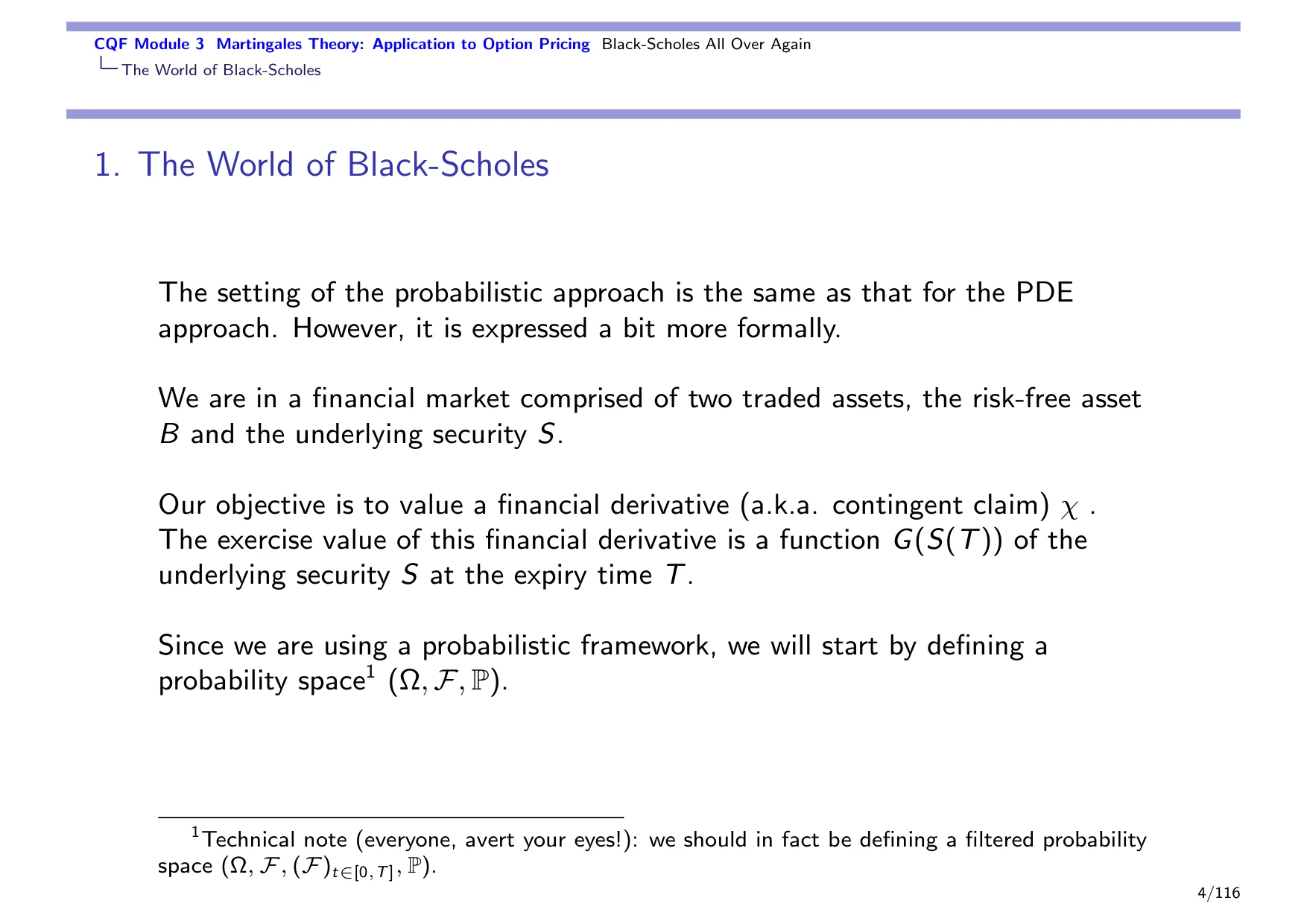
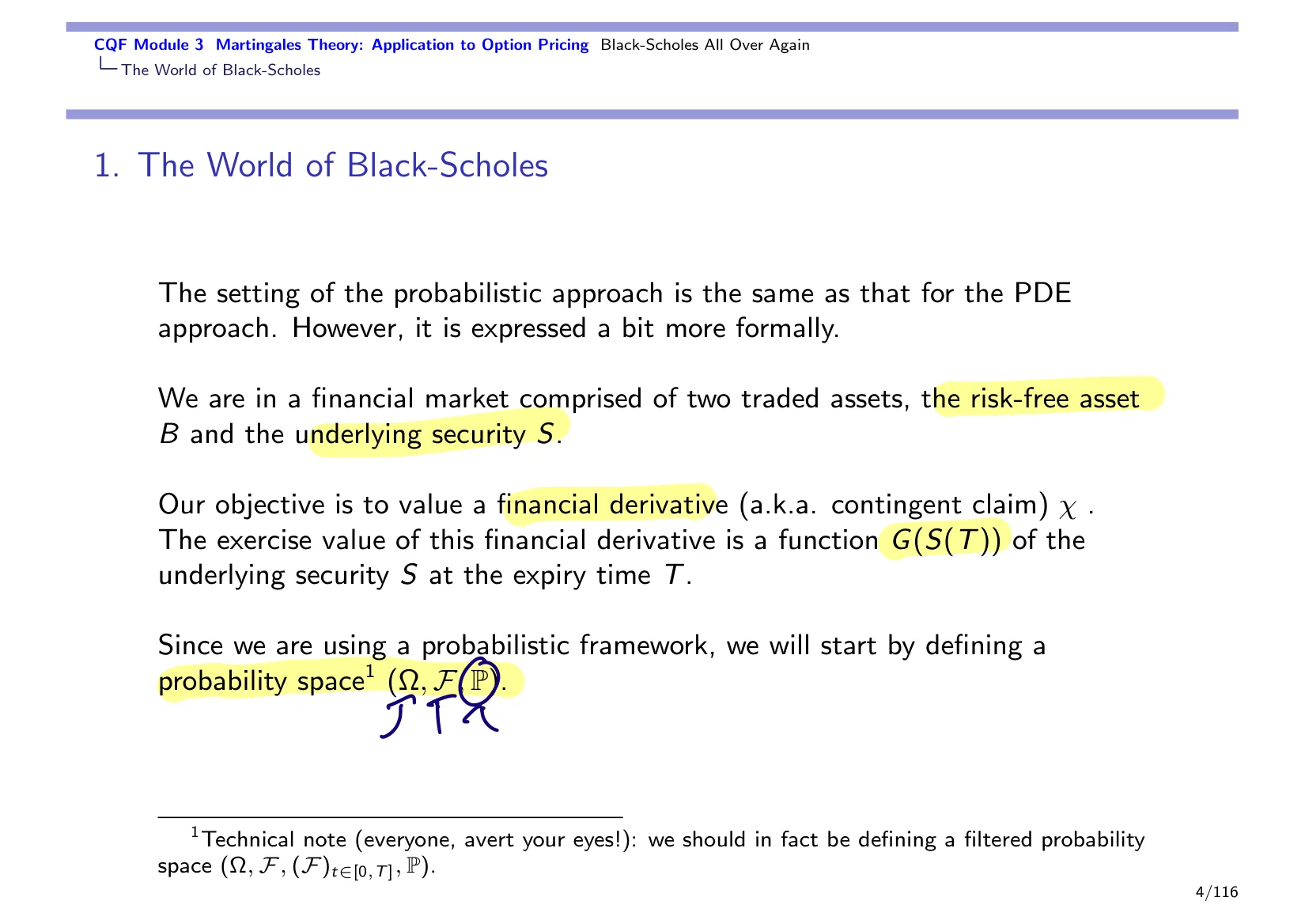
So I kept the notation simple and just putPut option An option that gives the holder a payoff when the underlying asset price falls below the strike. a little footnote. If you're not into technical stuff, just close your eyes, don't look at the footnotes.
This is where you're going to have something a bit more rigorous in the footnote, so avert your eyes if you're afraid of going for full filtered probability spaceProbability space The mathematical setting that contains outcomes, events, and probabilities for a random experiment.. Focus on the essential, which is that we've got a probability space, we have a set of events, the sample space omegaSample space omega The sample space Ω is the set of all possible outcomes of the experiment or model., we've got some information flow, that's the filtrationFiltration A time-indexed family of information sets describing what is known at each moment., and we've got probabilities. One thing that we're going to play around with is probabilities, and that's where the change of measure comes in.
For the rest, we have a risk-free rater / risk-free rate r is the risk-free rate used as the baseline interest rate in the model., a risk-free assetRisk-free asset A risk-free asset is an asset whose return is treated as certain in the model. as usual, and an underlying securityUnderlying asset An underlying asset is the asset that a derivative refers to and whose price helps determine the derivative’s value., which is the security on which our derivative, which in the literature is also called a contingent claimContingent claim A contingent claim is a derivative contract whose payoff depends on future market outcomes., is based. So we are trying to price these financial derivativesDerivatives Financial instruments whose value depends on the performance of another asset or variable., chi, whose payoffPayoff The payoff is the amount received from a contract or strategy, usually evaluated at maturity. is a function of the underlying at time big T. So exactly the same setup as Black-Scholes.
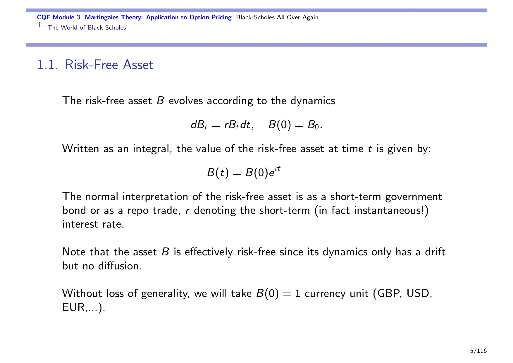
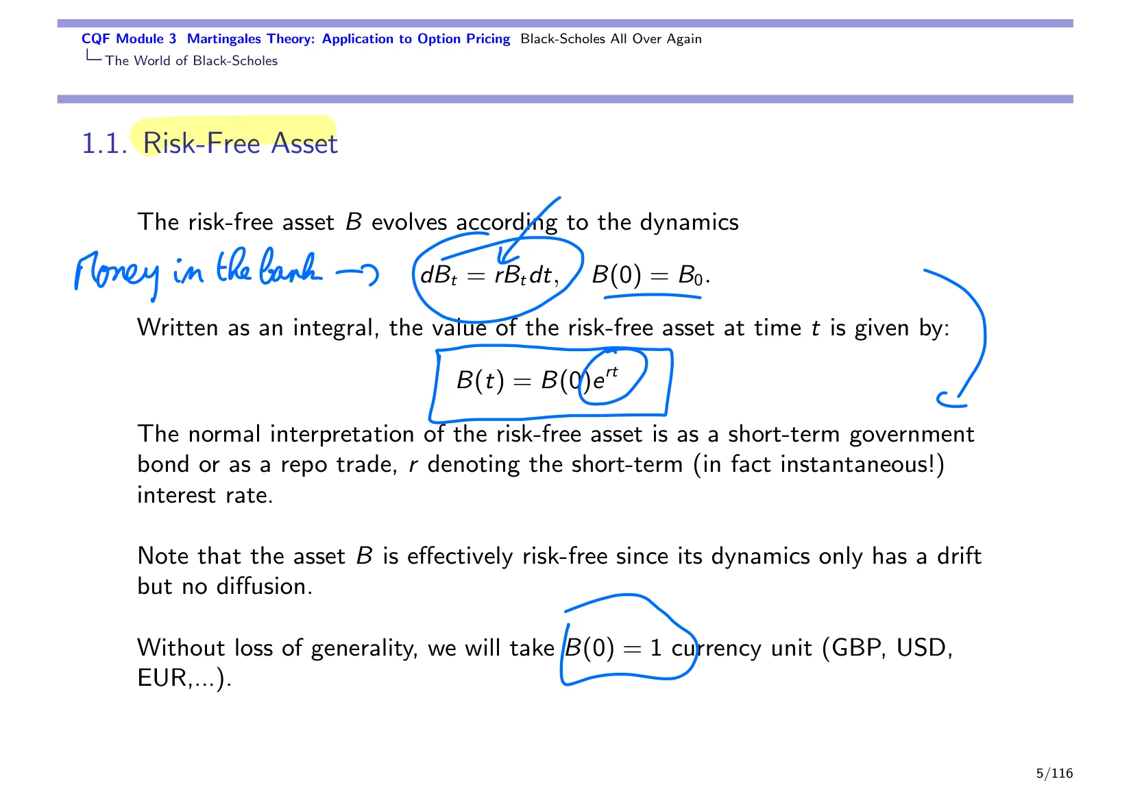
For the risk-free assetRisk-free asset A risk-free asset is an asset whose return is treated as certain in the model., we've got the risk-free dynamics, the money-in-the-bank dynamics, which is how interest compounds. You can see that this is just an ODE, where the risk-free rate is, of course, a constant because it's the risk-free rate. So you have a simple ODE to solve, and when you solve this simple ODE you see that money compounds in continuous timeContinuous time Continuous time is a modeling setting where variables evolve at every instant rather than at separate time points., giving you this e to the rt. The base amount is some arbitrary amount B0; without any loss of generality we take B0 to be equal to 1, one currency unit at time zero.
Now we bring in the underlying assetUnderlying asset An underlying asset is the asset that a derivative refers to and whose price helps determine the derivative’s value.. The underlying asset S is modeled through a geometric Brownian motionGeometric Brownian motion Geometric Brownian motion is a continuous-time stochastic process commonly used to model asset prices., the usual geometric motion that you now have learned how to manipulate and tame. dSt is equal to nu St dt plus sigma St dXt. This is your Brownian motion right there. The drift and diffusion coefficientDiffusion coefficient The coefficient multiplying the stochastic or random part of a diffusion model.s nu and sigma are constant.
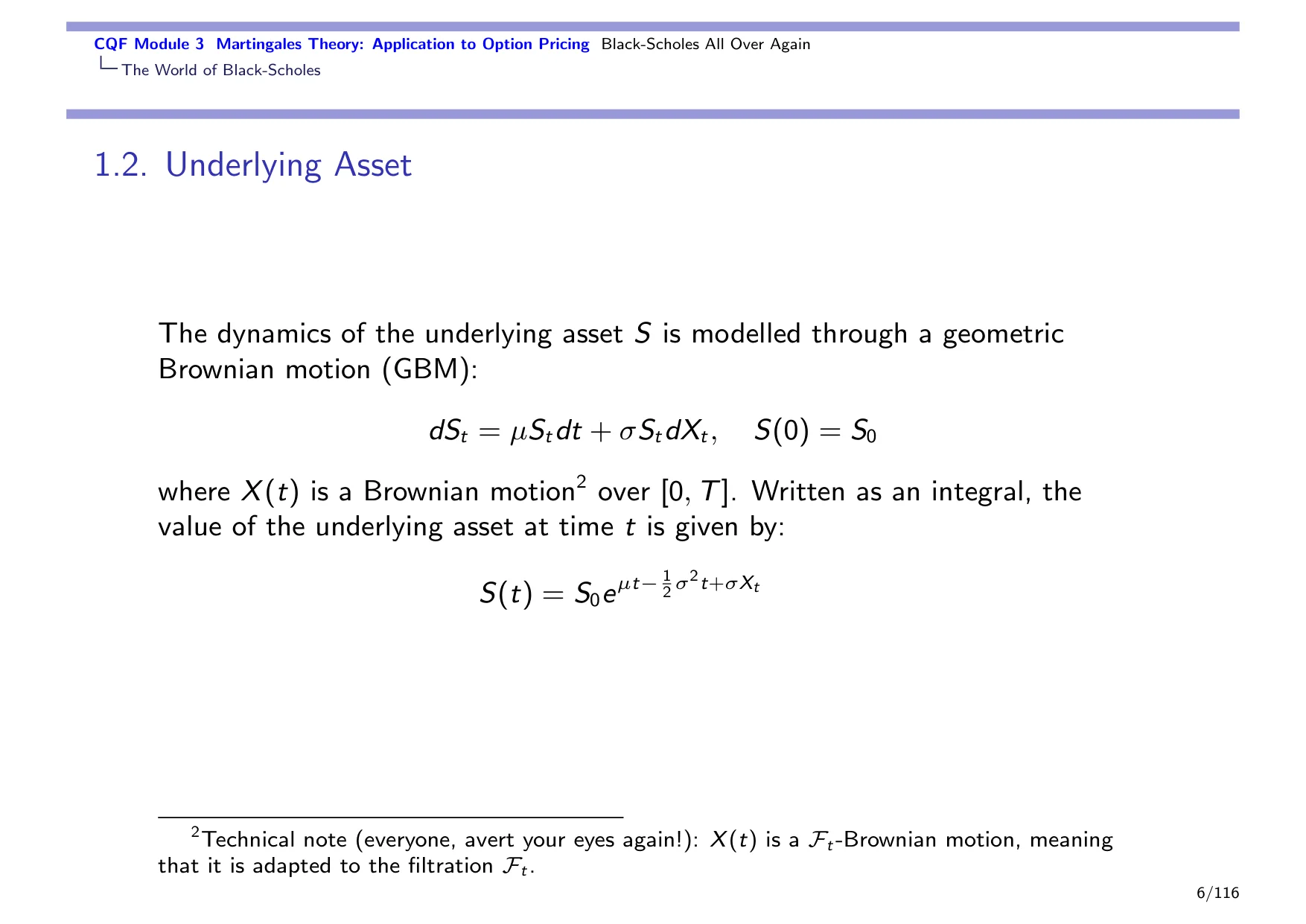
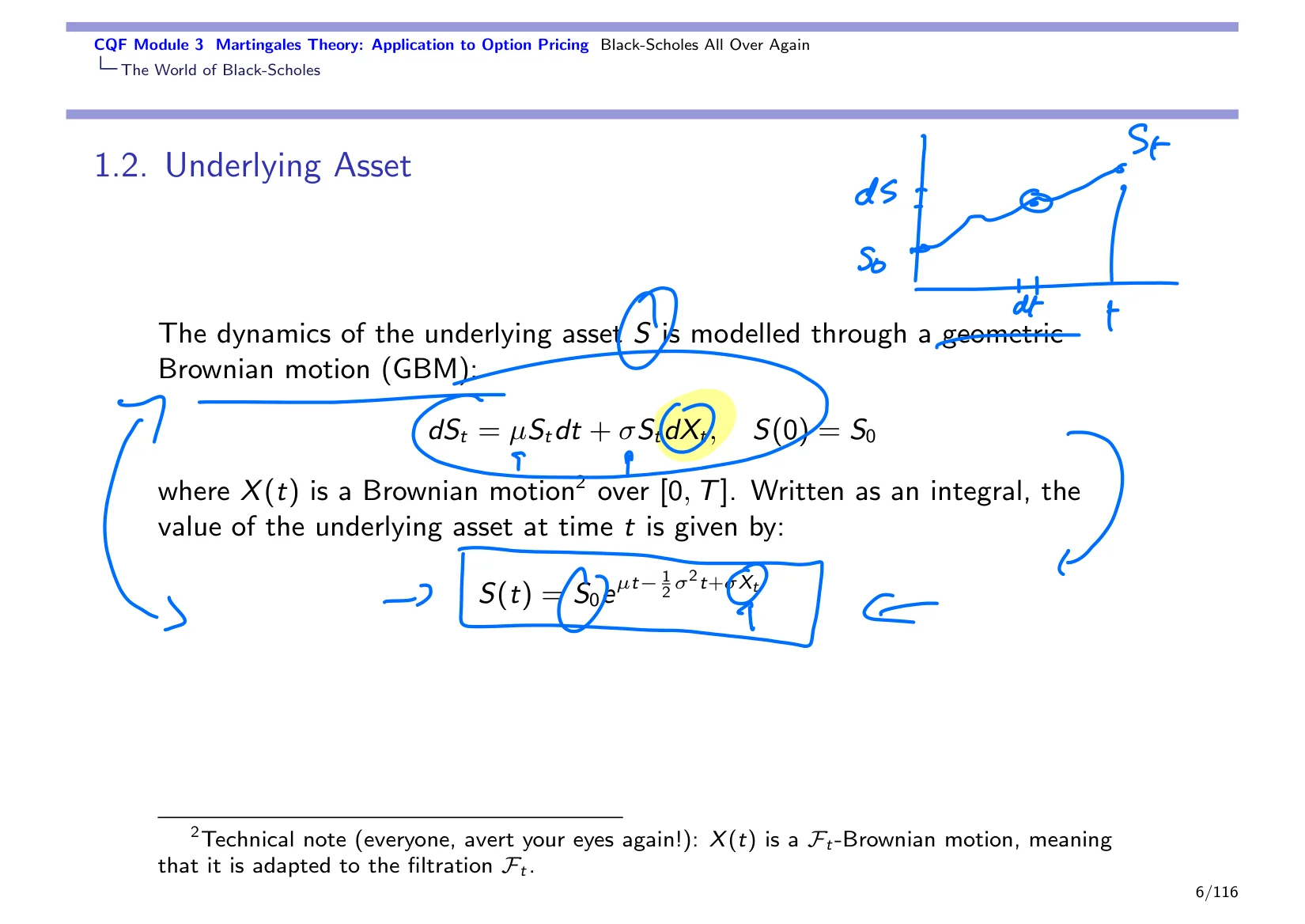
When you solve that SDE, you get this solution, so you can express the SDE as a solution, which is really the value of the process. Of course, the value of the process is random because it depends on Xt. In probability and in stochastic processes, we like to play around with the SDE and its solution. The reason is that, and that's something that will come back over and over again tonight and Thursday, the SDE, just like any differential equation, tells you about the motion in a very small time interval, in a little ball dt, and looks at how much the stock priceStock price The stock price is the current value of the stock at a given time. moves inside this little ball.
Now with the solution, you have a global approach where you know that your stock priceStock price The stock price is the current value of the stock at a given time. started at S0S0 / S*sub*0* S0 is the initial asset price at time 0. and you can just move it seamlessly to any time t without having to move one little ball at a time. So this is actually quite powerful to know the stock price at time t. Of course, you don't know the stock price exactly, but you can write down its equation, and you know that up to Xt you can write the rest of the dynamics. So this gives you a global view of where your stock price is going to be at some time t, and you can therefore manipulate the probability distributionProbability distribution A probability distribution describes how probability is assigned across possible outcomes of a random variable. from that perspective.
Now you have probably already used that when you did some Monte Carlo simulationMonte Carlo simulation Monte Carlo simulation is a numerical method that uses random sampling to estimate expectations or prices., or if you haven't, you will manipulate that when you do Monte Carlo simulation. You will learn that you're not going to need to simulate the evolution of your stock price every little dt when you are trying to price a European optionEuropean option An option that is exercised only at its expiry date.. You can directly go to the terminal valueterminal value Terminal value is the value of an asset, portfolio, or payoff at the final time in a model or calculation., and the terminal value will be given by something that's an application of this formula. You jump directly from where I am to where I'll be at the end, which computationally makes a lot of sense and saves you all the move up, move down, move up, move down, which you actually don't need if you've got a European option. You just need to know the terminal price, not how you got there.
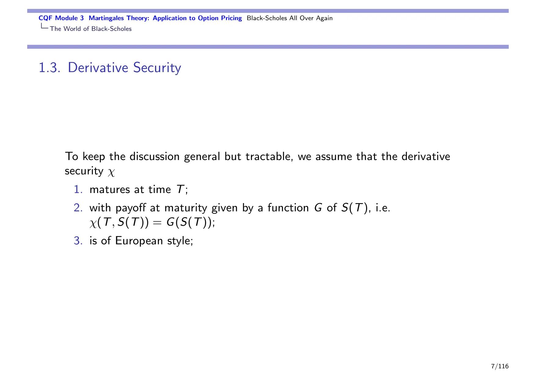
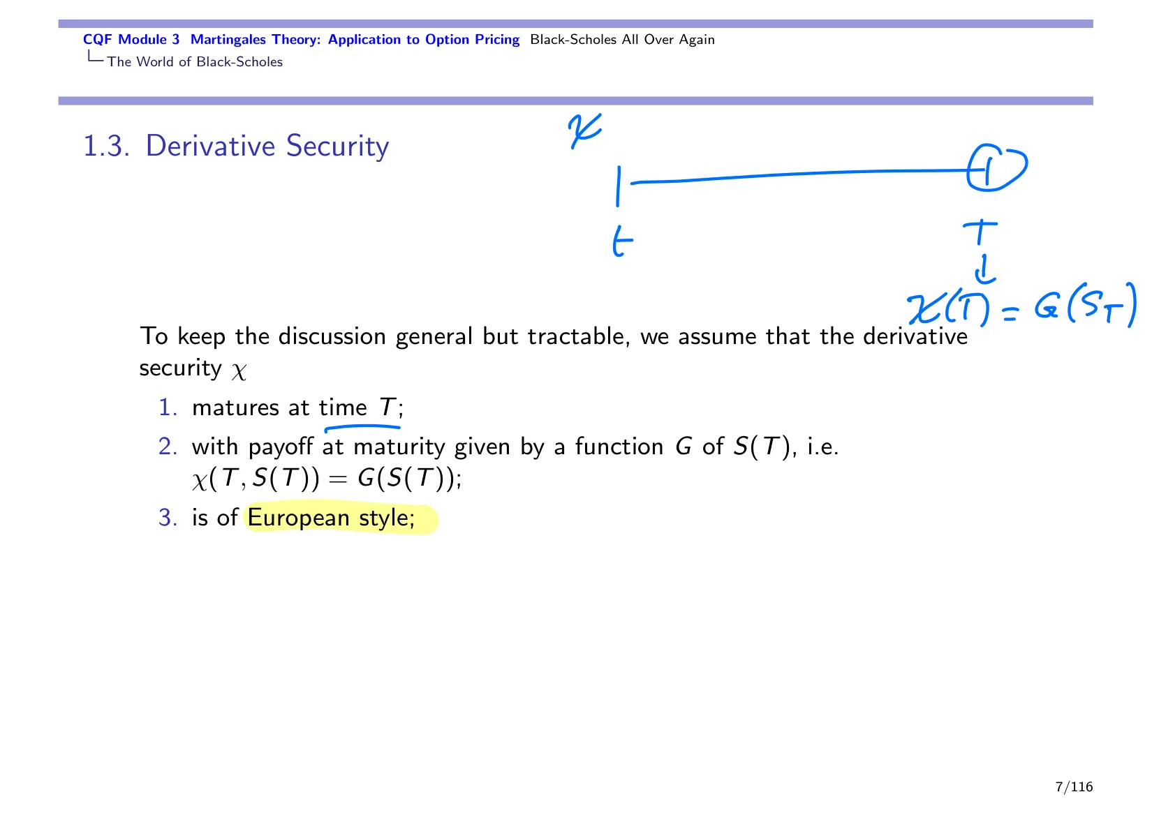
Now our derivative security matures at time big T, so right now we're standing here at time little t. We have a derivative that matures at time big T; it has a payoff at maturity. So the payoff at maturity, chi T, is just some function of your stock price at time big T, so S. That's the stock price; B is the bond priceBond price The bond price is the current value of a bond in the market.. So that's the difference here: your bond price, your risk-free asset, is risk-free, you see that it's governed by an ODE, but your stock price, the underlying asset, is risky. It has a term that depends on the Brownian motion; it is modeled using a stochastic differential equation. So those are the differences between S, the stock price, and B, the bond price.
Just like in the PDE approachPDE approach A pricing method that formulates the problem as a partial differential equation and solves for the option value., we should even be fairly consistent on the notation. Today we focus on European optionEuropean option An option that is exercised only at its expiry date.s, just like what you did with the PDE approach. Among the other assumptions, we're going to find all our favorites from portfolio selection. First, short selling is allowed. Two, the market is frictionless, which means that there are no transaction costsTransaction costs Transaction costs are the expenses or frictions associated with trading an asset., taxes, lack of liquidity, or constraints on short selling. As a consequence of one and two, the assets can be bought and sold, or even shorted, in unlimited quantity.
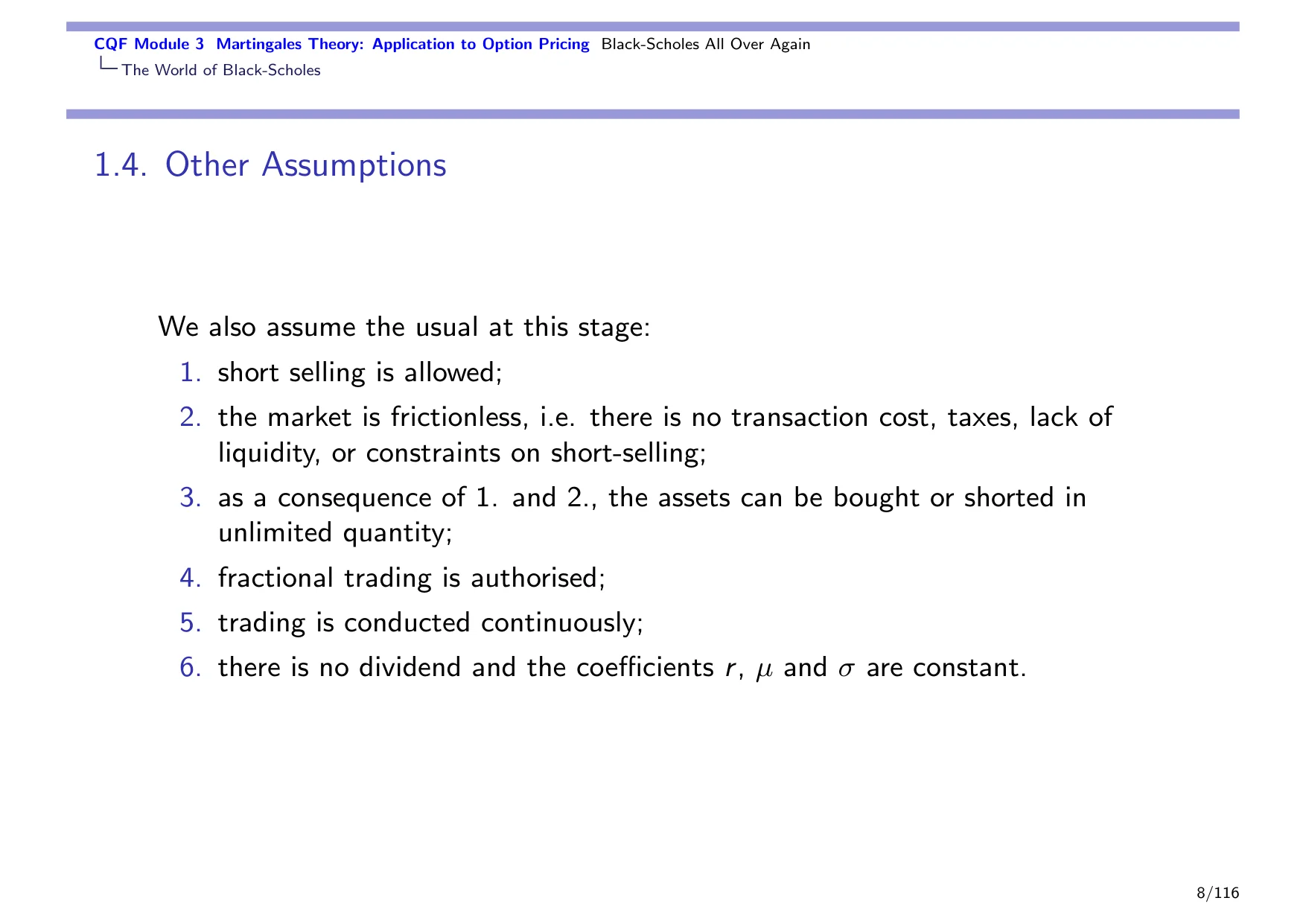
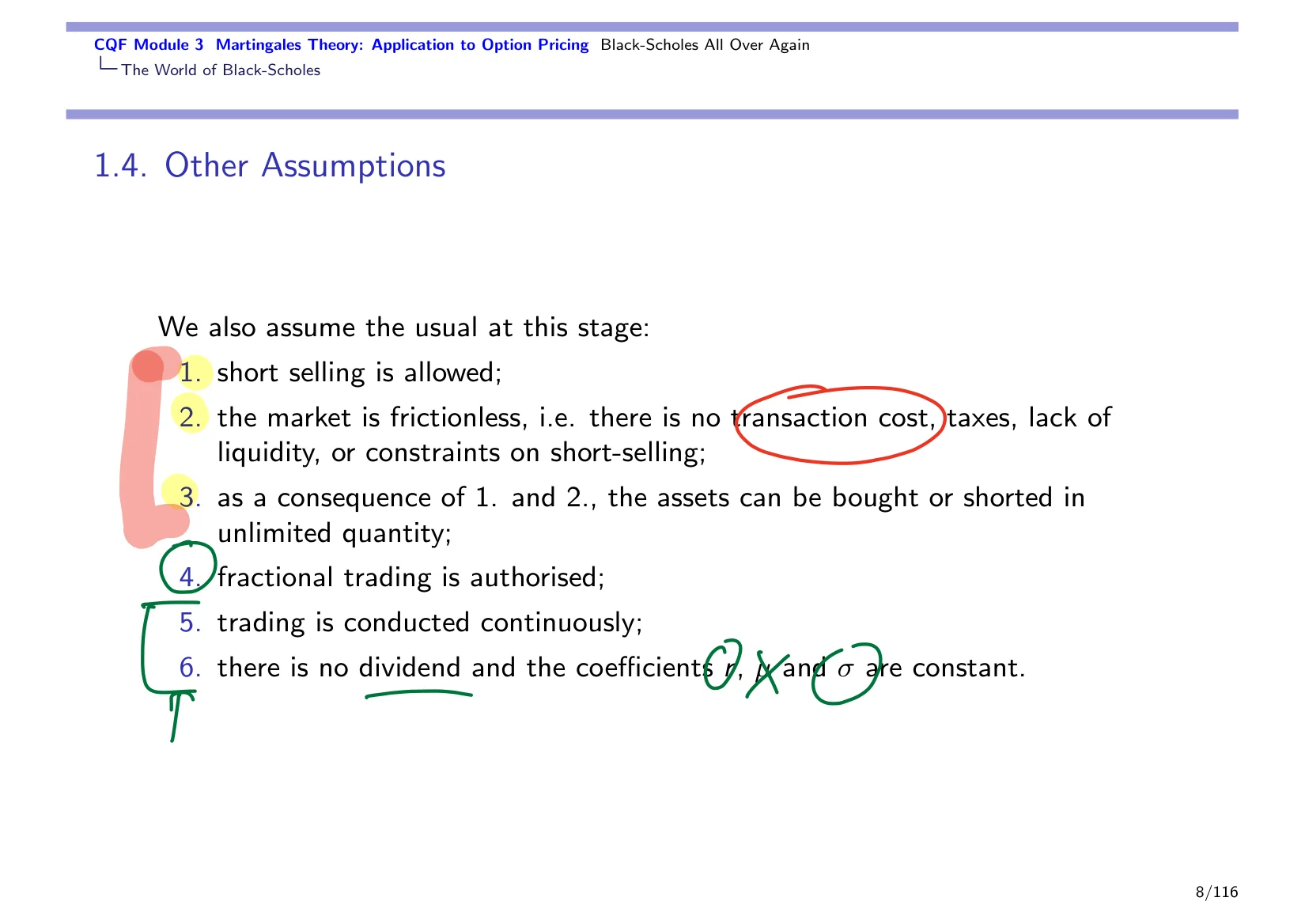
Of course, these assumptions here are totally unrealistic. However, they are a nice starting point if you want to get to a model that you can use. After that, of course, you will need to remove some of these assumptions, for example by adding transaction costsTransaction costs Transaction costs are the expenses or frictions associated with trading an asset.. I know that on the portal there's a wonderful lecture by Paul Wilmott about transaction costs. The model with PDEs is particularly elegant; there is a nice chapter in his book as well. So transaction cost is something that you will need to add later, and then we're still trying to get good models for liquidity, but this is actually quite hard.
Then we find an old favorite, which is that fractional trading is authorized. We were okay with it with portfolios; we're still okay with it now. Then the next two are really something that's proper to our setup in continuous timeContinuous time Continuous time is a modeling setting where variables evolve at every instant rather than at separate time points.. One, trading is conducted continuously. We are in continuous time; we can trade at any time when the market is open.
And six here, related to the model, and here again a decent first assumption when you want to get to a model, you've got to turn off a lot of bells and whistles. So no dividend coefficient; r, mu, and sigma are constant. Actually, we're going to see that we don't care much about mu in option pricingOption pricing Option pricing is the process of determining a fair value for an option from its payoff and model assumptions.. Dividends are constant; we can reintroduce the dividends later, that's not a problem.
r is constant. As early as the 1970s, we start to find the first models that say, wait a second, r can be stochastic; that's the Vasicek modelVasicek model The Vasicek model is a mean-reverting stochastic model for interest rates., and that's just a few years after Black-Scholes. So the assumption that r is constant, which was necessary for Black-Scholes, got removed pretty quickly after that. And sigma is constant: this is something that was removed later, starting in 1987 for the first few papers, and then 1993, where we start to consider stochastic volatilityStochastic volatility Stochastic volatility is volatility that changes randomly over time.. So it took much longer to consider stochastic volatility than stochastic interest ratesStochastic interest rates / stochastic interest rate Stochastic interest rates are interest rates that vary randomly over time., but slowly we removed some of these assumptions. We have models with transaction costs now, we have models with stochastic interest rates, we have models with stochastic volatility by now.
Okay, here is where we are going to go. Bond priceBond price The bond price is the current value of a bond in the market. is present valuePresent value The current worth of a future cash flow after discounting it back to today. of strike. In which book? If you're referring to the Black-Scholes formula, yeah, we have a term, the term that's in front of the N of d2N(d2) / N of d2 N(d2) is the standard normal CDF evaluated at d2., is the present value of the strike. Present value is the same formula as a zero-coupon bondZero-coupon bond A zero-coupon bond is a bond that pays only its face value at maturity and no interim coupons., because the zero-coupon bond, as you will see in module four, is actually the present value of one currency unit, pound or dollar, paid later.
You're going to see that in module four.
We're just doing everything with the risk-free rate, so our interest rates are constant. The mathematics of compounding, so to go to the future, that's the future value, which is what we do with B right now, and of discountingDiscounting The conversion of a future payment into its present value., which we'll do later, which is getting the present valuePresent value The current worth of a future cash flow after discounting it back to today. of a future payment, are very closely related. We'll explore that a bit later in the lecture tonight, but hold on for actual bond prices until you get to Module 4, because that's when you're going to see stochastic interest ratesStochastic interest rates / stochastic interest rate Stochastic interest rates are interest rates that vary randomly over time., and that's when things really start to get more interesting.
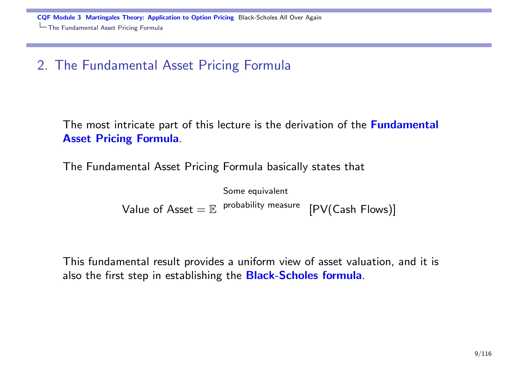
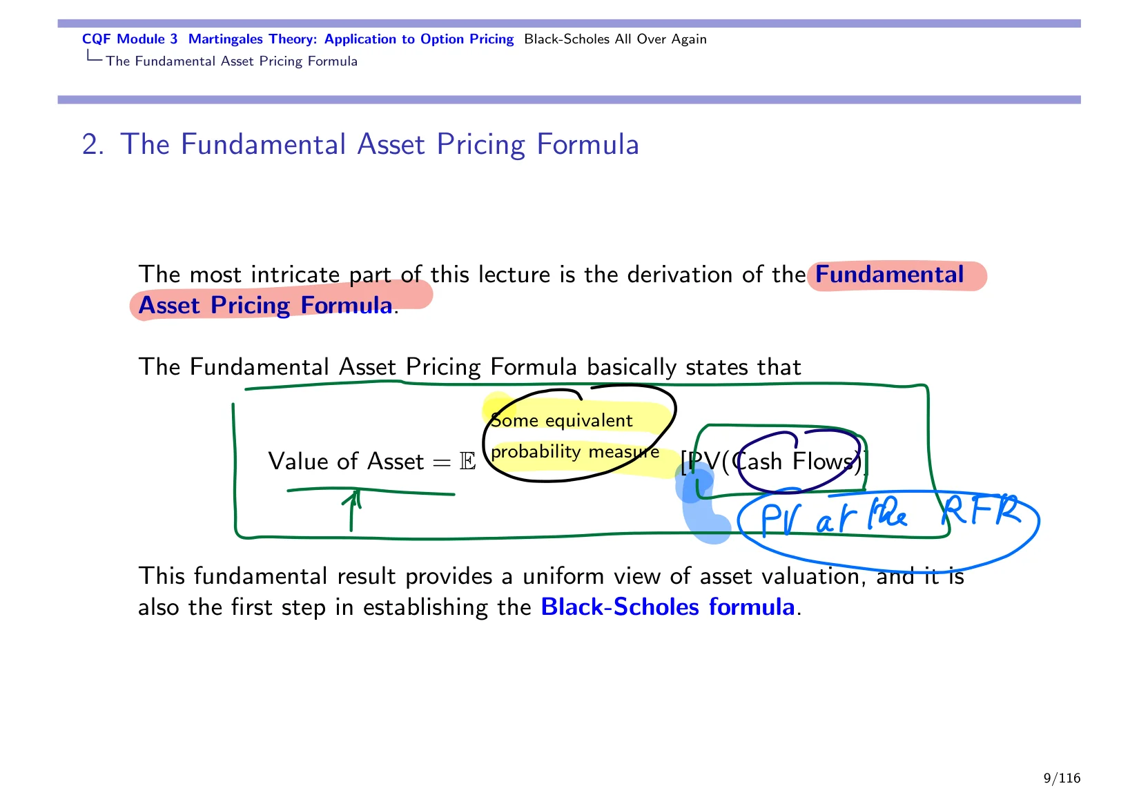
Where we're going to go tonight is this: the first and key result, the one that we really want to show, and that actually corresponds to the Black-Scholes PDE in more ways than one, is this fundamental asset pricing formula. The fundamental asset pricing formula tells you that the value of an asset, actually of any asset, can be calculated as an expectation of the present value of your future cash flowsCash flows Cash flows are the payments or receipts generated by an asset or contract over time.. But there is a little twist: the expectation is not in the physical, real-world measurePhysical measure P / measure P Physical measure P is the real-world probability measure used to model observed asset behavior.. It's not with respect to probabilities that we've got in the real world, not with respect to probabilities that we use, for example, for trading or portfolio management.
We need to tweak these probabilities in order to be able to compute the value of the asset as an expectation, and that's what we're going to do today: find the right tweak for the probabilities, the right reweighting, the right change of measure, or change of variable, depending how you want to code it, in order to be able to compute the value of an asset simply as an expectation of its future cash flowsCash flows Cash flows are the payments or receipts generated by an asset or contract over time.. When I say present value of the future cash flows here, the present value that we're going to use today is the present value just using our risk-free rate, present value at the risk-free rate. It's not necessarily at the risk-free rate in general, and that's something we discuss later in the lecture when we talk about change of numeraireChange of numeraire A change of numeraire is a pricing method that switches the reference asset used to measure values. and the numeraire technique, but in Black-Scholes and in a lot of other option pricing approaches, we're actually going to look at the present value using the risk-free rate.
This formula is important because, when you open it up and try to understand what it does, it is actually the formula that is at the heart of Monte Carlo simulationsMonte Carlo simulation Monte Carlo simulation is a numerical method that uses random sampling to estimate expectations or prices.. That's also why this formula is fundamental. It's fundamental because even if you don't solve the expectation, even if you don't compute the expectation, by the time you can write down your fundamental asset pricing formula, you can then implement it numerically using Monte Carlo methods.
Let's imagine that you want to price a call option. Your stock price is here with a starting value of S0S0 / S*sub*0* S0 is the initial asset price at time 0.. Your time horizon is there, that's big T, and let's add your strike priceStrike price The strike price is the fixed price at which an option can be exercised.. Your strike price is somewhere there; that's your strike price, your exercise price. What this formula is telling you is that first you're going to compute the cash flows, then you will present-value them, and as these cash flows are random, you're going to have a distribution of cash flows, so what you do is you take the average, the expectation.
Let's imagine that we already know what probability system we want to be in. What this formula is telling us is that if you cannot solve the formula analytically, you just simulate. You simulate a path for S, and then another one, then another one, and then another one, and then another one, etc. So you simulate a whole truckload of paths for S, and of course by the time you're done with your thousand, ten thousand, hundred thousand simulations, you will get a nice distribution for S. So this is S at time T; now that's the distribution for S.
What you want to price is a call option, so we need to look not at the distribution of the stock price but at your payoff, because your payoff is your cash flow. As the strike here is set at this level E, we know that any stock price that ends up below the strike gives you a payoff of zero, so here you're going to have a big probability mass exactly at zero. That's all these occurrences here that get ported away to your payoff. The payoff starts at zero, and then you've got the rest of your distribution, which is ST minus E for ST greater than E. So all we are doing is applying this function, max of ST minus E or zeroCall payoff / max of ST minus E or zero A call payoff is max(ST − E, 0), the amount paid by a call option at maturity., to the stock price to get the distribution of payoff.
Now we've got the cash flows from our option, so the next step is to take these cash flows and then present-value them, so bring them back to time zero, when we started. So bring back this entire distribution and move it down to this time, and after that you just take the average present value of your cash flows. Then you just take these values and average them, and that's, in a sense, what Monte Carlo does. Monte Carlo methods apply strictly the fundamental asset pricing formula. They use it as a recipe in order to generate prices, asset prices, derivative pricesDerivative prices The values assigned to derivative contracts, often computed as an expected discounted payoff., from a distribution of stock prices under an appropriate probability measureEquivalent probability measure / appropriate probability measure An equivalent probability measure is a new probability measure that preserves which events are impossible, while changing their probabilities otherwise., so with appropriately tweaked probabilities.
If you've done Monte Carlo simulation for option prices, you will have seen that actually we don't use mu as a drift; we use r. We are using risk-neutralQ / risk-neutral Q is the risk-neutral measure used in pricing and hedging calculations., and we are going to see tonight how we derive these risk-neutral probabilities and this risk-neutral dynamicsRisk-neutral dynamics Risk-neutral dynamics are the model equations for asset evolution under the risk-neutral measure.. The bottom tail, which goes negative, is all ported back to zero because what we care about are the cash flows. The cash flows for an option start at zero; it's the maximum of ST minus E or zero. Therefore your minimum cash flow is zero. That's why we don't care about that: all this stuff where ST ends up below E gets ported to zero, and that's why we've got this big spike in the probability distribution at zero.
Why not average first, then take the present value? You could do that as long as your interest rates are deterministic, but as soon as your interest rate becomes stochastic, you can't do that. So that's why we take the cash flows, we take the present value, and then we average. This is a much more general method than averaging first and then taking the present value. Averaging and taking the present value only works with deterministic interest ratesDeterministic interest rates Interest rates that are assumed to be known in advance and not random..
Is this a form of importance samplingImportance sampling Importance sampling is a Monte Carlo technique that improves estimation by drawing samples from a more convenient distribution and adjusting the weights., where we change from real to neutral then? Yes, actually importance sampling is a great example of a change of measure. We use change of measure in option pricing; we use them in some portfolio management problems, risk-sensitive investment management problems. So I basically change measure for a living, among other things, and yes, it's also at the heart of importance sampling. Importance sampling is a change of measure.
A putPut option An option that gives the holder a payoff when the underlying asset price falls below the strike. would be the mirror image. You could do the same thing with a put, except that your function for a put would be maximum of E minus ST or zeroPut payoff / maximum of E minus ST or zero A put payoff is max(E − ST, 0), the amount paid by a put option at maturity., but it's the same approach. So you would just average the cash flows that you get with your put. I illustrated it with the call; you can do the same thing here.
For a put, that would look something like this, very roughly. This is T. You've got your stock price that goes and diffuses merrily. Your distribution of stock prices at time T is lognormalGeometric Brownian motion Geometric Brownian motion is a continuous-time stochastic process commonly used to model asset prices., so a long fat tail on one side and a short tail on the other. Then when you map that to your put payoffPut payoff / maximum of E minus ST or zero A put payoff is max(E − ST, 0), the amount paid by a put option at maturity., let's say that your strike is here, that's your strike, then anything that's above gets mapped to one big probability mass at a payoff of zero, and then your payoff for a negative run turns positive in the opposite direction.
It's basically this tail that you get here, but just shifted a bit as E minus S_t. Here you see your payoff. I've inverted the scale, so what I've done is basically minus S_t minus E to be able to represent it and just show you where the tail went, but that's the same thing. So that's what happened with the put. Your tail goes there. No, no, no: the bottom tail does not become negative, because it's E minus S_t, so it's minus S_t minus E, right? So you re-center and you flip the sign. You see it works. It still works with put. Isn't that wonderful? I think it is.
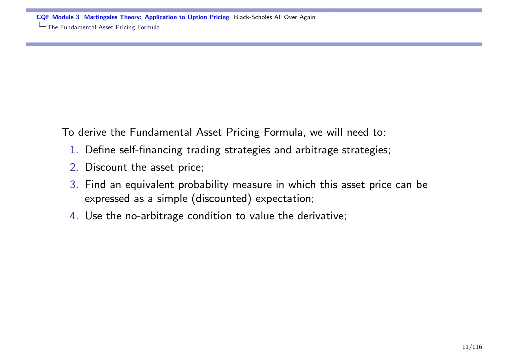
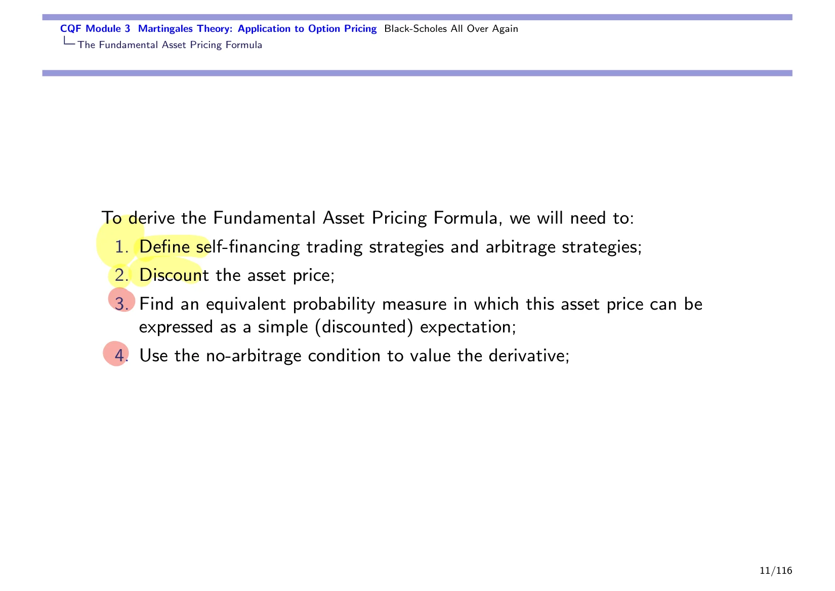
I've talked about Monte Carlo simulation, so how are we going to get to this fundamental asset pricing formula? I wanted to show you the result as a motivation to get there, because we have to go through four steps. The first one is, and that's an unfortunate consequence of dealing with complicated mathematical objects, we need definitions. We need to define precisely what we mean by the type of trading strategiesTrading strategy / trading strategies A trading strategy is a rule for how to hold and rebalance assets over time. that we're going to adopt, and we also need to be precise in terms of what we mean by arbitrageArbitrage Arbitrage is a trading strategy that yields a sure profit without requiring an initial investment or exposing the trader to risk., which is something that we did not need to do with PDEs, as PDEs are local.
As long as you do something reasonable, you don't really need to define what you're doing, because the error of doing something unreasonable over a very, very tiny ball around your current point is negligible. So you can basically treat everything as pretty much as in the deterministic case. But here we can't. We have to embrace probabilities, which means we have to have some definitions. So that's number one.
Number two, and that's actually quite simple, although I put a few slides on that, we discount the asset price. DiscountingDiscounting The conversion of a future payment into its present value. means that we keep the dollar value of our stock constant. We remove inflation, and to do that we just remove the natural growth of interest rates, so we consider discounted asset pricesDiscounted asset prices Asset prices adjusted for the time value of money by dividing by a discount factor. because naturally in finance asset prices inflate over time.
That's inflation working. Inflation pushes prices up: prices of physical goods, but also prices of financial goods. However, all the results we've got in mathematics and physics consider that we don't have this phenomenon of inflation, so we need to deflate our pricesDeflate prices / deflate our prices To deflate prices means to divide prices by a reference asset or discount factor to simplify valuation. before we can really use them properly mathematically, and that's what we do. We just discount them.
This is standard stuff in finance in order to make sure that you can look at asset prices in constant dollar terms, meaning when you see, for example, prices expressed in economic time series, you see that it's all based on 1990 dollars, for example. So that helps you understand whether prices have really increased because the intrinsic value of the good has increased, or if it was just an effect of inflation. So here we're always going to discount asset prices in order to make sure that an asset price later is comparable to an asset price now.
Then we get into the thick of it. We find an equivalent probability measureEquivalent probability measure / appropriate probability measure An equivalent probability measure is a new probability measure that preserves which events are impossible, while changing their probabilities otherwise., meaning we find a neat way of tweaking our probabilities so that we can benefit from all the nice properties of martingales and expectation. Then we wrap things up using the no-arbitrage conditionNo-arbitrage condition A market pricing condition that prevents riskless profit opportunities from inconsistent prices. to value derivativesDerivatives Financial instruments whose value depends on the performance of another asset or variable., and we will have a fundamental asset pricing formula.
But if we know that they are impacted by inflation, why do we take that away? Our mathematical results don't look at inflation, so we would need to incorporate inflation everywhere in our model, which makes the model heavier. So the best way is just to remove inflation, and you will see that anyway when you remove inflation you get back to talking about things that we've seen in portfolio theory, which is the risk premiumRisk premium A risk premium is the excess return required for taking on risk., which also makes much more sense because you really want to know how much your stock is increasing with respect to the risk-free rate, not just how it is increasing in nominal terms.
And yes, we are going to go to a different environment where we can price things much more easily, and yet the price that we get will still be valid here in this world, which is actually the true little miracle of this approach.
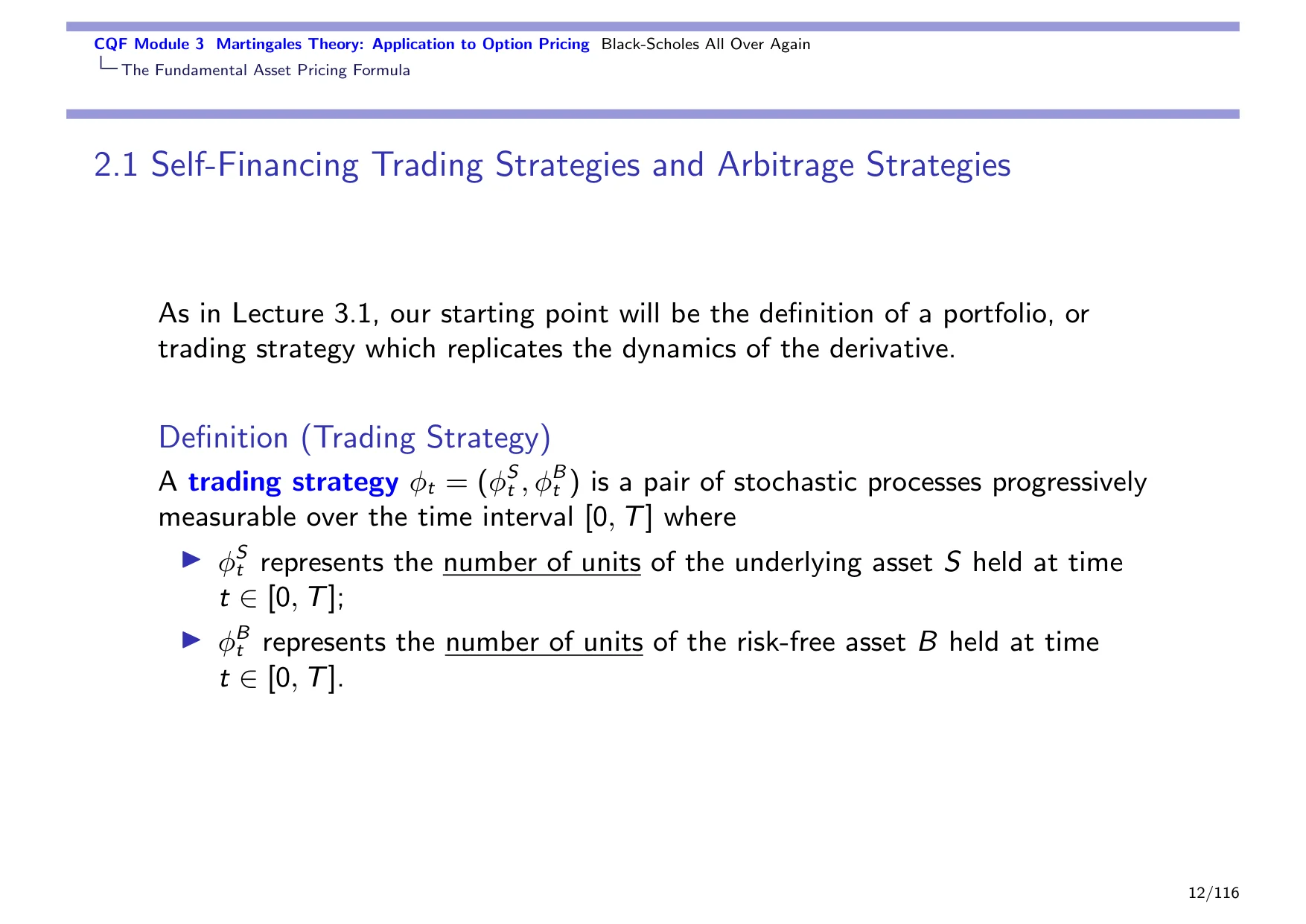
Okay, so let's start with our definition. The first one is that of a trading strategyTrading strategy / trading strategies A trading strategy is a rule for how to hold and rebalance assets over time.. You remember when you did the PDE, you set up a hedged portfolioHedged portfolio A hedged portfolio is a portfolio arranged so that its value is less sensitive to market risk.. Here we're going to do the same thing. We are going to set up a trading strategy to mimic, to recreate, the option payoffOption payoff The cash flow or value an option produces at maturity, determined by the underlying asset price.. That's what we call a replicating portfolioReplicating portfolio A replicating portfolio is a portfolio constructed to match the payoff of another asset or derivative..
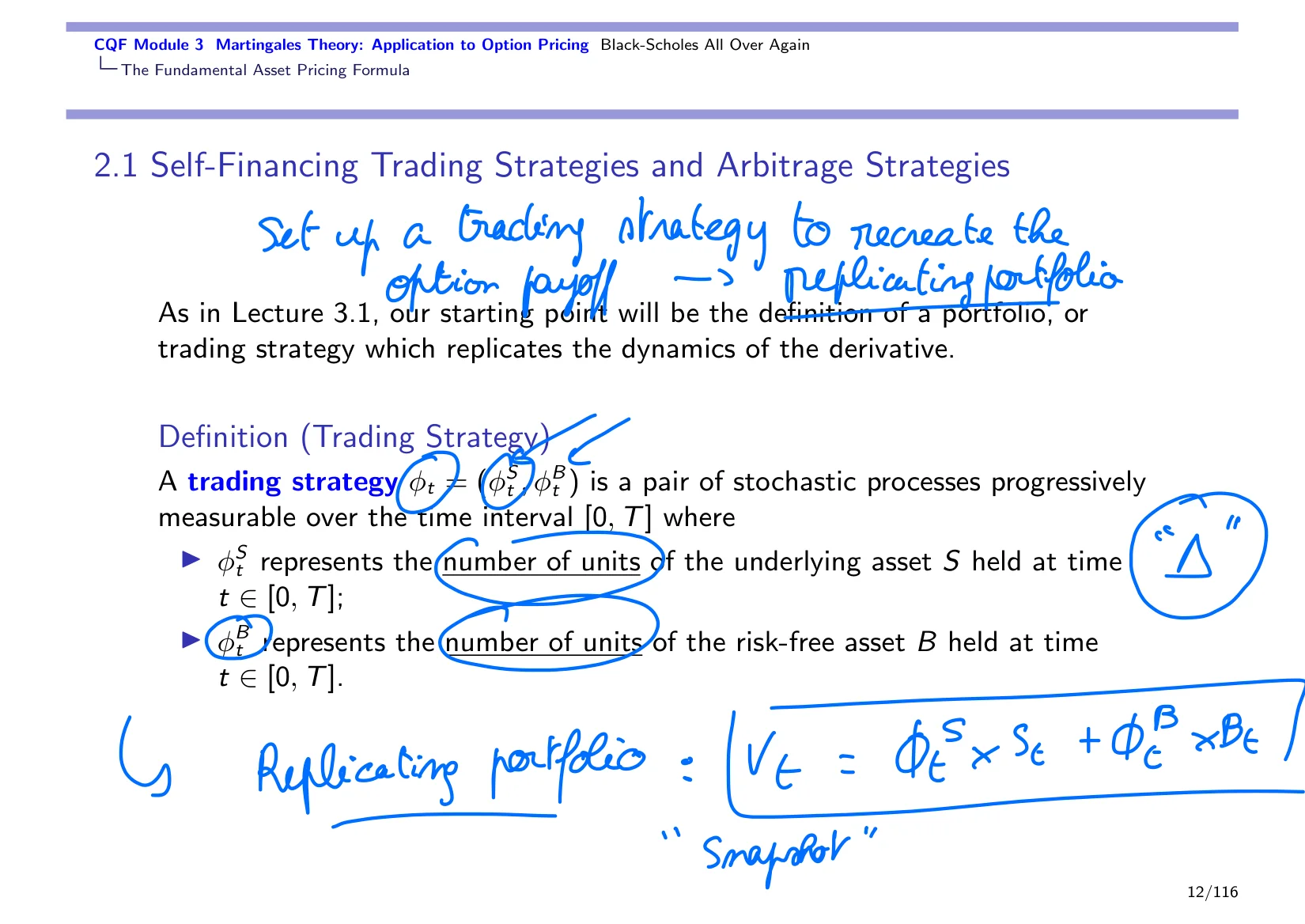
This is closely connected to what you've seen in terms of hedging portfolio, because the replicating portfolioReplicating portfolio A replicating portfolio is a portfolio constructed to match the payoff of another asset or derivative. is just a short position in the hedging portfolio. So, for example, if you sell a call and you want to hedge that position in the call that you sold, you're going to buy stock. Now, if you wanted to create this short option position, you would need to sell stock. Your replicating portfolio for that should be short stocks.
So the replicating portfolio is very closely linked; it's just the opposite sign of the hedging portfolio that you had before. Now, this trading strategy rests on two things. It's actually a process with two values. It's a pair of stochastic processes, with one value that represents the number of units of underlying asset S that you're trading, so that's your deltaDelta Delta is a sensitivity measure, usually the derivative of an option price with respect to the underlying asset price. from PDE, and the other value, phi_t^Bphi / phi_t^B A notation for a trading strategy or integrand in a stochastic integral, depending on the context. in this case, represents the number of units of the risk-free asset that you hold at time t.
So a trading strategy is a pair of processes, and of course it's stochastic because as the stock price changes you're constantly readjusting your delta. That's something you've learned from PDE, so you're constantly readjusting how many stocks you've got in your portfolio. Therefore the number of stocks in your portfolio is random, and it's connected to the stock price.
So that gives you this trading strategy, telling you that your replicating portfolio, the portfolio that's supposed to mimic, to recreate, the option, has a value V_t that's just the number of shares that you own times the stock price plus the number of units in the bond, in the risk-free asset, times the value of the risk-free asset, of your bank account, at time t. And this is what I call the snapshot equationSnapshot equation The snapshot equation is the equation describing the portfolio value at a given time..
It's a snapshot equationSnapshot equation The snapshot equation is the equation describing the portfolio value at a given time. because it tells you, at time t, the value of your replicating portfolio is that. Tell me how many shares you've got, tell me how many units you've got in the bank account, I look at the share price, I look at the value of the bank account, I put that together, and that's the value of your replicating portfolio. It doesn't tell me how things evolve in time, but it tells me precisely what the value of your replicating portfolio is at time little t. So that's our trading strategy.
Now we have to limit a little bit the scope of trading strategies that we are going to consider. One of the reasons for that is that we want to keep things simple, meaning that we don't want to have to track cash flows coming in and out of our trading strategy. We just want to focus on our trading strategy and make sure that by trading bonds and stock all the time with the same pot of money, we can recreate the same payoff as the option.
We don't want to have to track how much money we put at the end of the month to reflate the strategy, capitalization, and we don't want to have to track how much money we take out, which is consumption. So we're not going to consider any intermediate cash flow. We set up a pot of money and then we use that pot of money to recreate the option payoffOption payoff The cash flow or value an option produces at maturity, determined by the underlying asset price., and that's what we call a self-financing portfolioSelf-financing Self-financing means a portfolio is rebalanced without adding or withdrawing external cash..
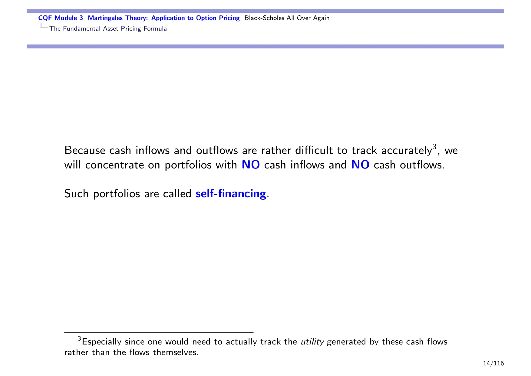
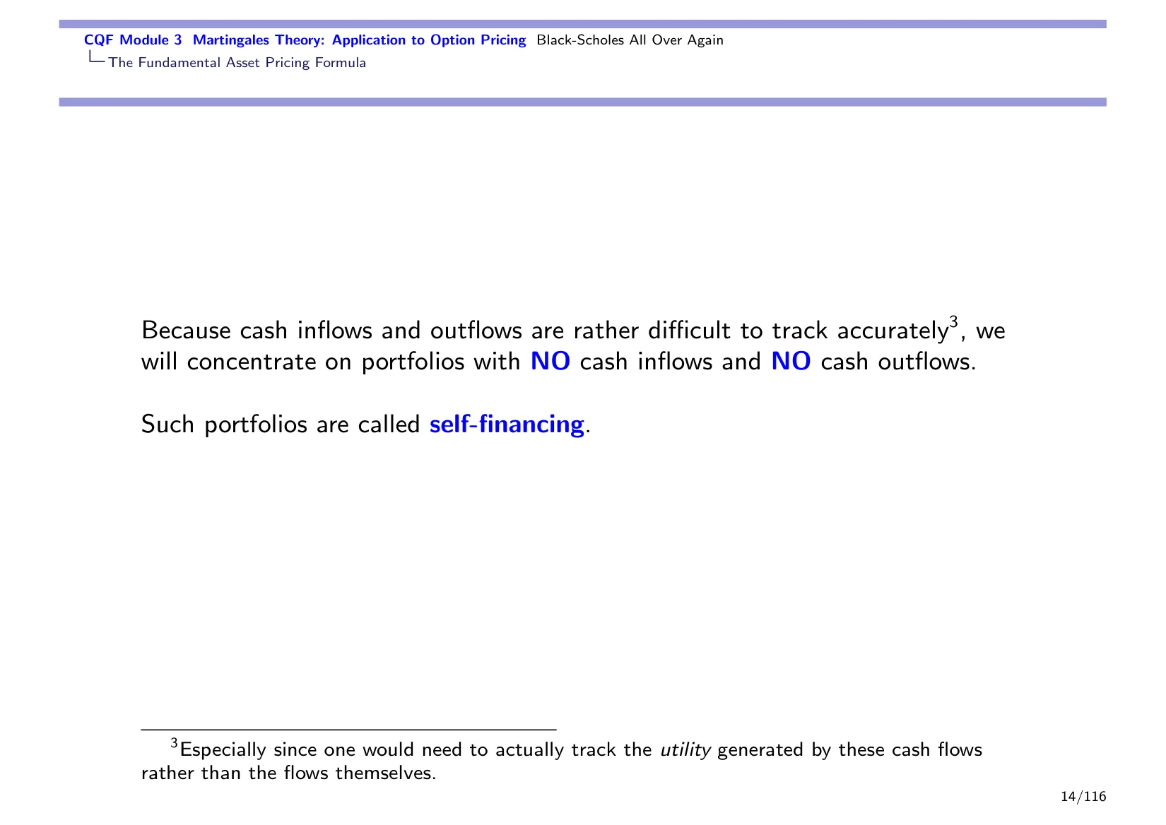
Self-financingSelf-financing Self-financing means a portfolio is rebalanced without adding or withdrawing external cash. because once we put the pot of money together, we don't add money to it, we don't take money away from it, we just trade whatever we've got. So of course the question that we face today is: how much money do we put in our pot? Because the amount of money that we put in our pot needs to be able to replicate, through smart trading, exactly the payoff of the option we're trying to price.
So the restriction on self-financing trading strategies is that they are a trading strateg-
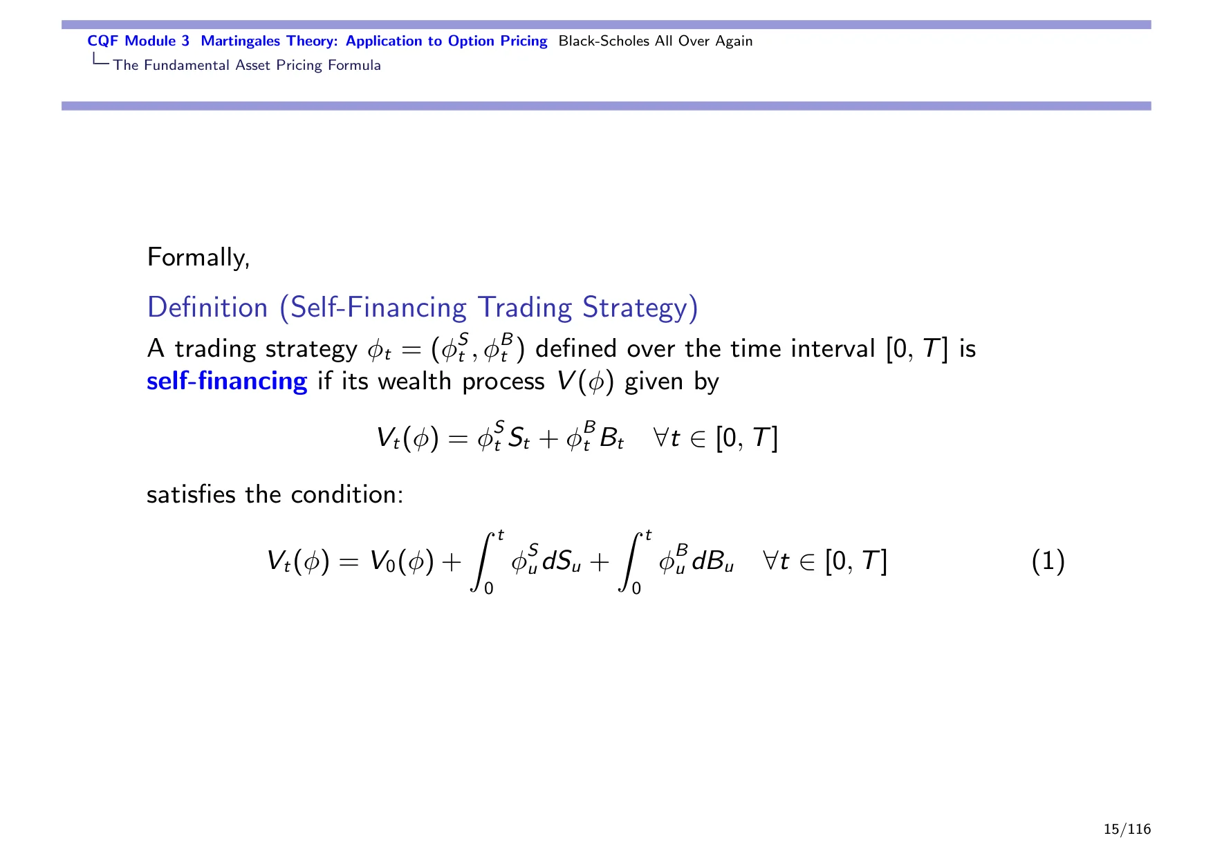
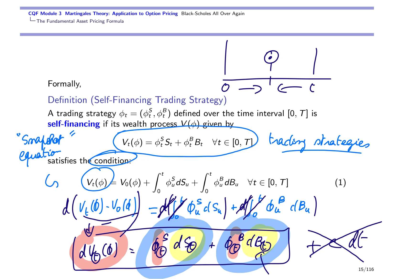
How much money do we put in our pot? The amount of money that we put in our pot needs to be able to replicate, through smart trading, exactly the payoff of the option we're trying to price. Remember, that's my snapshot equation for a trading strategy.
All trading strategies satisfy this snapshot equation, which is that at time t, the value of my portfolio is how many shares I've got times the share price, plus how many units of risk-free asset I've got times the value of each unit in the risk-free asset. But then we had one condition, which is the self-financing condition: the evolution of the risk-free asset, of my pot of money, of my self-financing strategy, depends solely on the evolution of the stock price and bond price.
To see why that's important, we're going to take the differential. We're going to convert this stochastic equation into a stochastic differential equation to see what happens at the atomic scale when time moves by just a little bit. To do that, you subtract V0 on both sides of the equation, so that gives you this equation here: the integral from 0 to t of phi_uphi / phi_t^B A notation for a trading strategy or integrand in a stochastic integral, depending on the context. dS_u plus the integral from 0 to t of psi_upsi / psi_u A notation for an integrand or strategy process in a stochastic integral, depending on the formula. dB_u.
Then what we do is take the differential, and of course the differential cancels the integral. What the differential does to this difference here is that, as we shrink the gap between Vt and V0, we get dVt. Putting back the notation into something consistent, we get dVt = phi_t dS_t + psi_t dB_tSelf-financing equation / dVt = phi_t dS_t + psi_t dB_t A portfolio condition saying its value changes only through the assets it already holds., where we are consistent in our notation for time.
All we've done is take this big equation that works between time t and time 0 and shrink it, and look at what's happening in a small neighborhood around some point in time. What this is telling us is that the change in the value of your portfolio right there actually depends on the change in the stock price and the change in the bond price, holding, metaphorically speaking, the number of assets constant for just a little dt.
We are exactly in the same setup as what you did when you created your replicating strategy with Black-Scholes for PDEs. You set the number of shares that you want to trade, and then you look at how the portfolio evolves on the little scale of dt, and that's exactly what we've got here.
This is important in terms of telling us that this portfolio is self-financing, because we see that the entire dynamics, the entire change in the value of the replicating portfolio, can be due to only two components: the change in stock price and the change in bond price. We do not add something, for example some amount that we add to the portfolio; we don't have that. We don't take any amount out of the portfolio either. Everything that's in the portfolio stays in the portfolio. We just reorganize it differently between stock and bonds, and over a very small time interval the only change in the portfolio value comes from a change in the stock price and from the natural compounding of interest in the risk-free asset.
Phi is just a random variable; it's a stochastic process. It's stochastic because the share price changes over time, therefore the number of shares you need to hold changes over time. That's what you learned with the PDE approach, when you learned that actually delta changes all the time. Here, what you call delta, we call it phi.
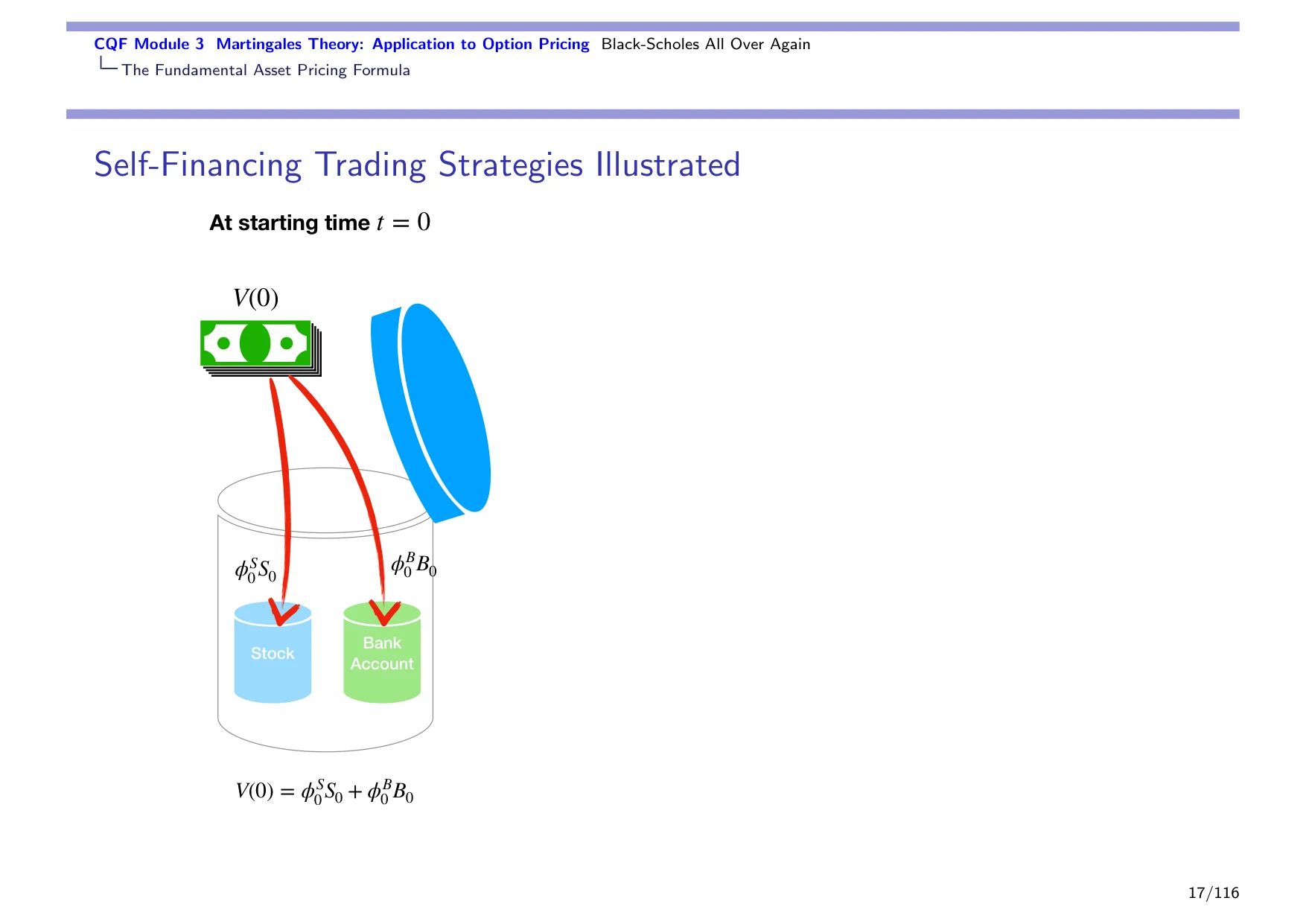
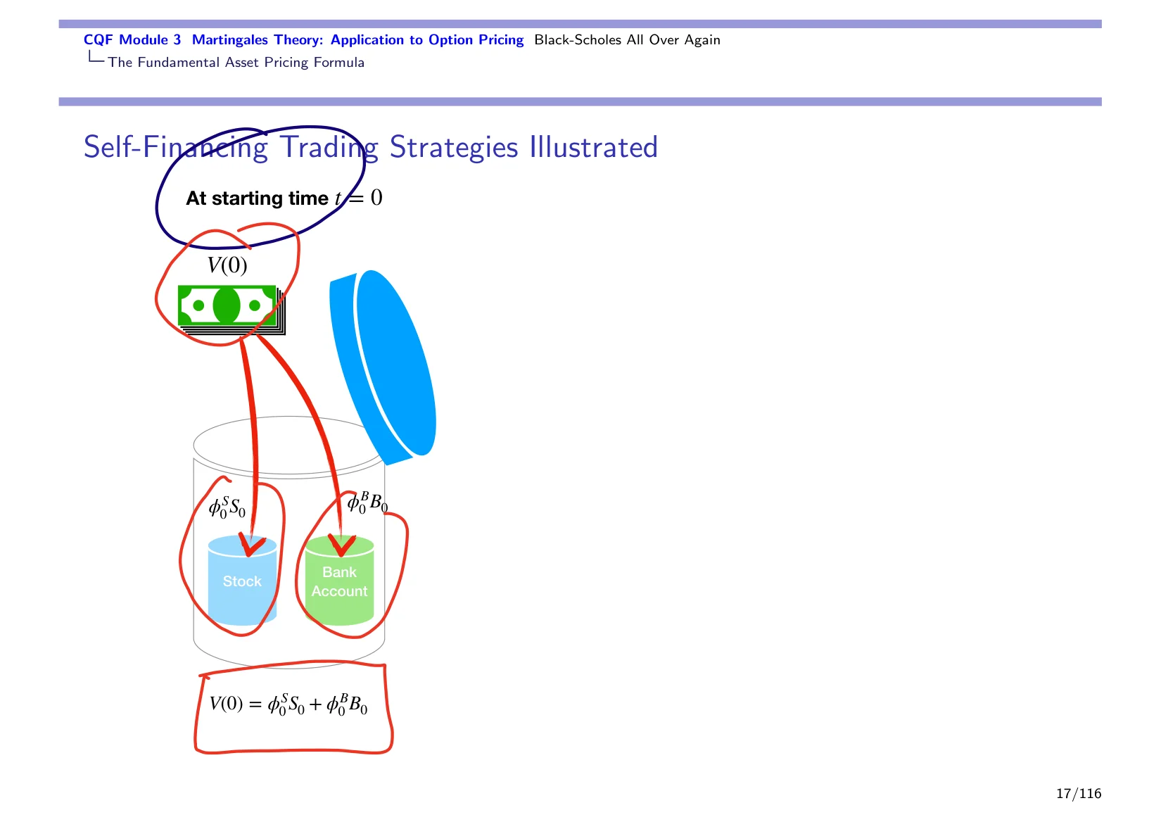
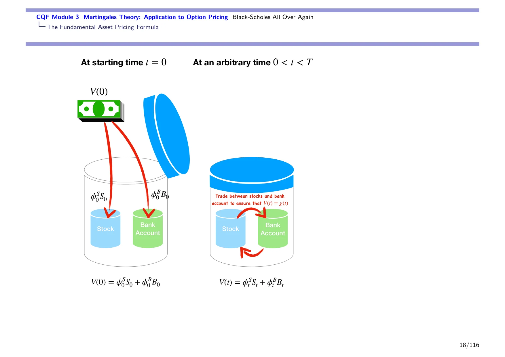
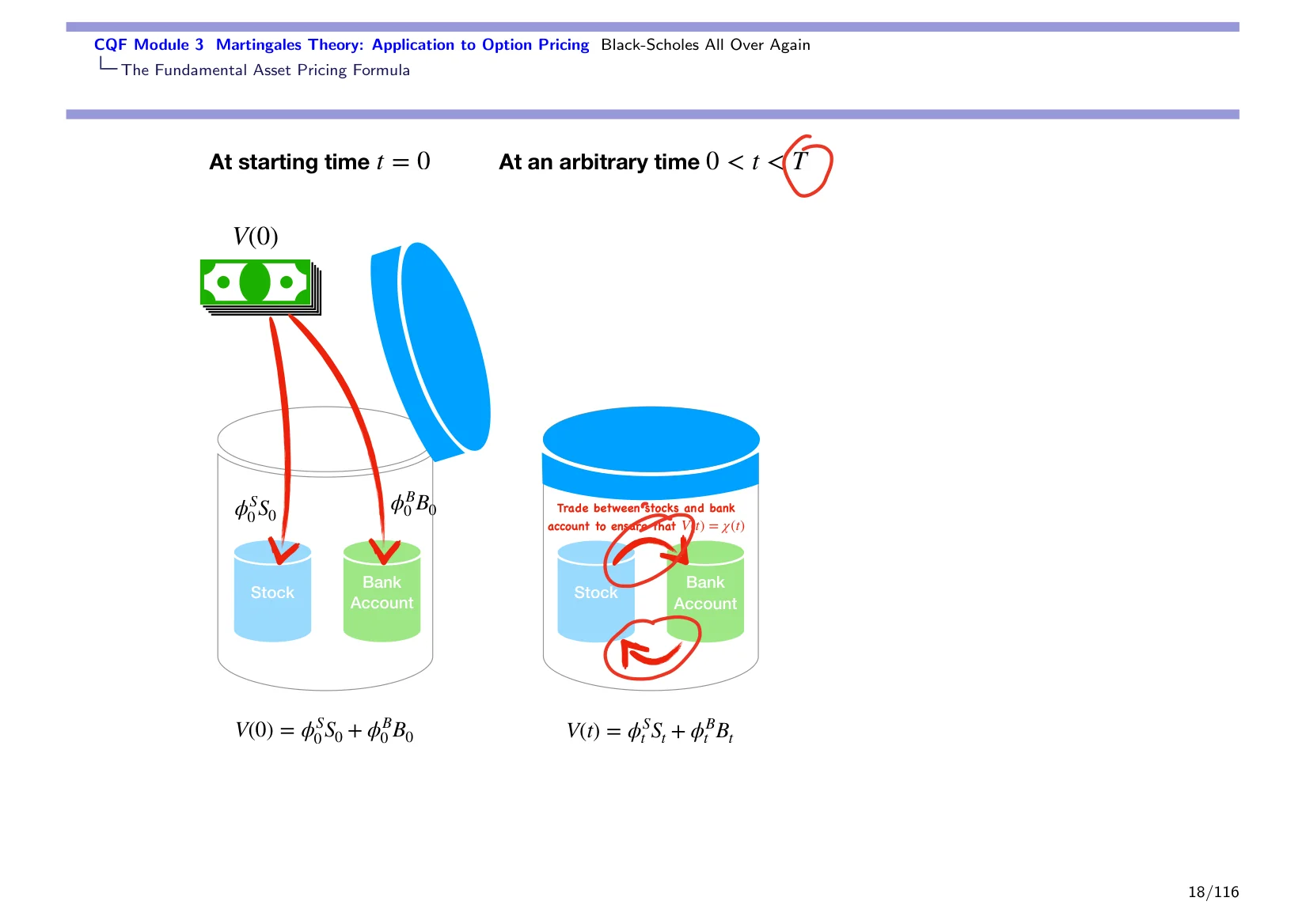
To illustrate what we've done with our self-financing trading strategies, I've got a little picture. That's our pot of money. We start at time t = 0. We put an amount of money inside the pot, split between stocks and bank accounts, so you see that at time 0 this is the value of our portfolio. That's using the snapshot equation.
Then as time goes, and before we reach expiryT / expiry T is the expiry time, meaning the maturity date of the contract. of our option, the pot of money is closed, and all we can do is just sell some of the stocks to put the money in the bank account, or take money from the bank account and put it in the stocks. We keep that flow going because the objective is that at expiry time, t = T, we want the money that we get, so the proceeds of the sale of our replicating portfolio, V_T, should be exactly equal to the payoff of the option in all states of the world. So we should match it exactly and always.
We need one more little definition, and then we can really be on our way. That definition is actually a plus for us: it's the definition of arbitrage. We're doing probabilities, so we're going to be a little bit more realistic in our approach to arbitrage. We're going to consider that an arbitrage opportunity is a trade.
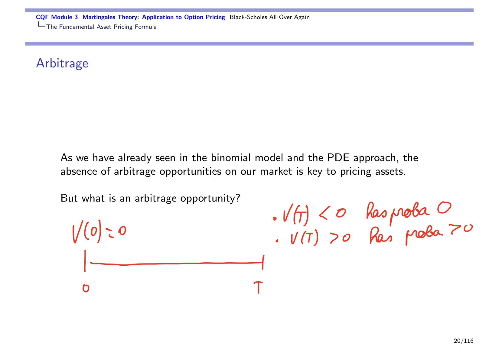
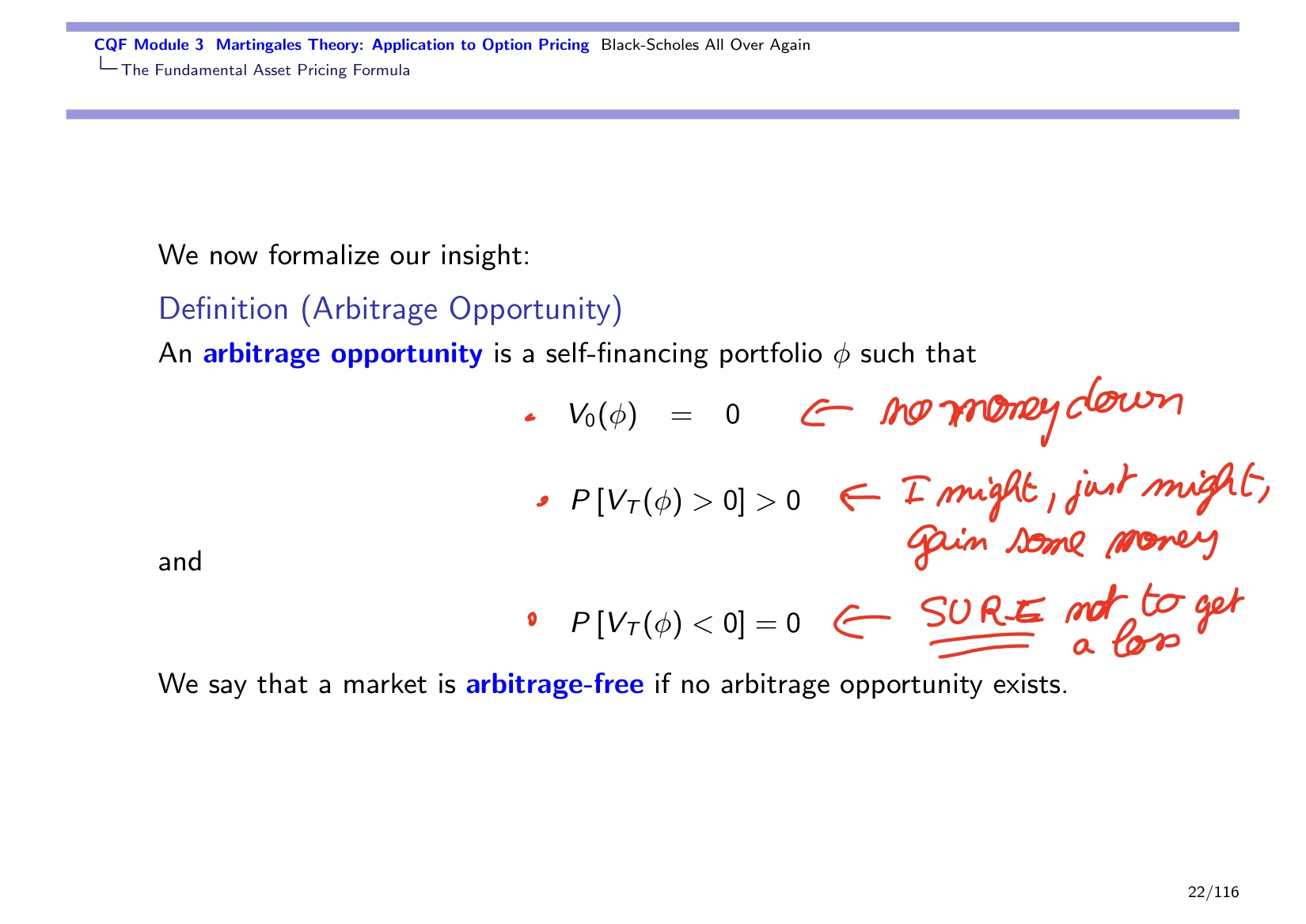
A trade where at time 0, I put no money down. I'm not committing any capital to a trade. I go into something long, short, for example, but the bottom line is I do not put any of my money in the trade at time 0. Then I wait up until some time T.
If there's an arbitrage opportunity, then I'm not losing any money for sure, meaning that the probability that my terminal valueterminal value Terminal value is the value of an asset, portfolio, or payoff at the final time in a model or calculation. is negative is zero. I am sure I won't lose any money, but V_T might just be positive. All I require is that there is some chance, some probability, that I might even make some money.
Think about it in terms of arbitrage. That means that you know that you're not going to make a loss and, on average, the expected value of your portfolio will be positive. So we can translate that definition of arbitrage into three rules: no money down, I might just gain some money, and I am sure not to lose money. That's what defines an arbitrage opportunity for us today.
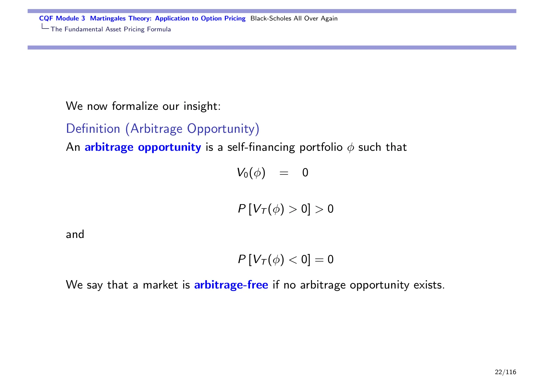
Notice that we're a little bit more realistic than what you see in the PDE approach or in the binomial modelBinomial model The binomial model is a discrete-time model where an asset price moves up or down by fixed factors over successive steps., where an arbitrage opportunity is: I don't put any money in and I am sure that I'm going to make some money later. When you start to incorporate probabilities, you can be more realistic.
By modern standards, this is not even considered very realistic. We've got more realistic models of arbitrage, such as no free lunch with vanishing riskNo free lunch with vanishing risk No free lunch with vanishing risk is a no-arbitrage condition ruling out nearly riskless profit opportunities., which really help us zoom in and narrow down realistic arbitrage opportunities. This one is still quite close, but it's progress with respect to what you've seen with the binomial model or the PDE approach.
That's the magic of arbitrage. That's why it's called an arbitrage opportunity. Arbitrage opportunities normally should not exist in financial markets. But at times they might, if prices are very much disconnected. You could have a trade where you borrow some money, you invest it, and then at the end of the period, you make some money.
Carry tradesCarry trade A carry trade is a strategy that seeks profit from differences in funding and investment returns. are an example of arbitrage. There are carry trades that can last for a long time, for example between currencies, especially when some countries are trying to defend their currencies very hard. They might actually underwrite a carry trade where traders find it advantageous to exchange their home currency against another currency, put that currency in a bank account, then collect the interest rate, bring the currency back to their home currency, and make money like that.
It's actually the central bank that is underwriting this carry tradeCarry trade A carry trade is a strategy that seeks profit from differences in funding and investment returns..
Underwriting this carry trade is an example of an arbitrage opportunity, but it never lasts very long because central banks cannot defend their currencies forever. We saw an example of that during the Asian crisis in 1997. There were quite a few carry trades going on, and when they collapsed, that contributed to the crisis.
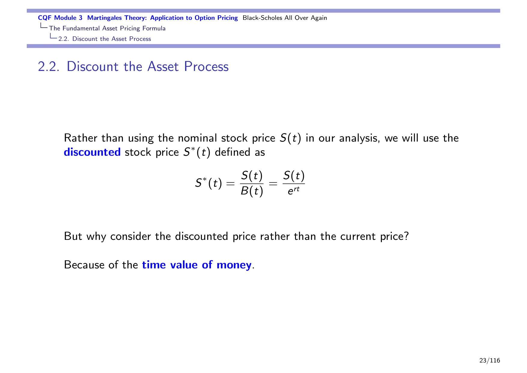
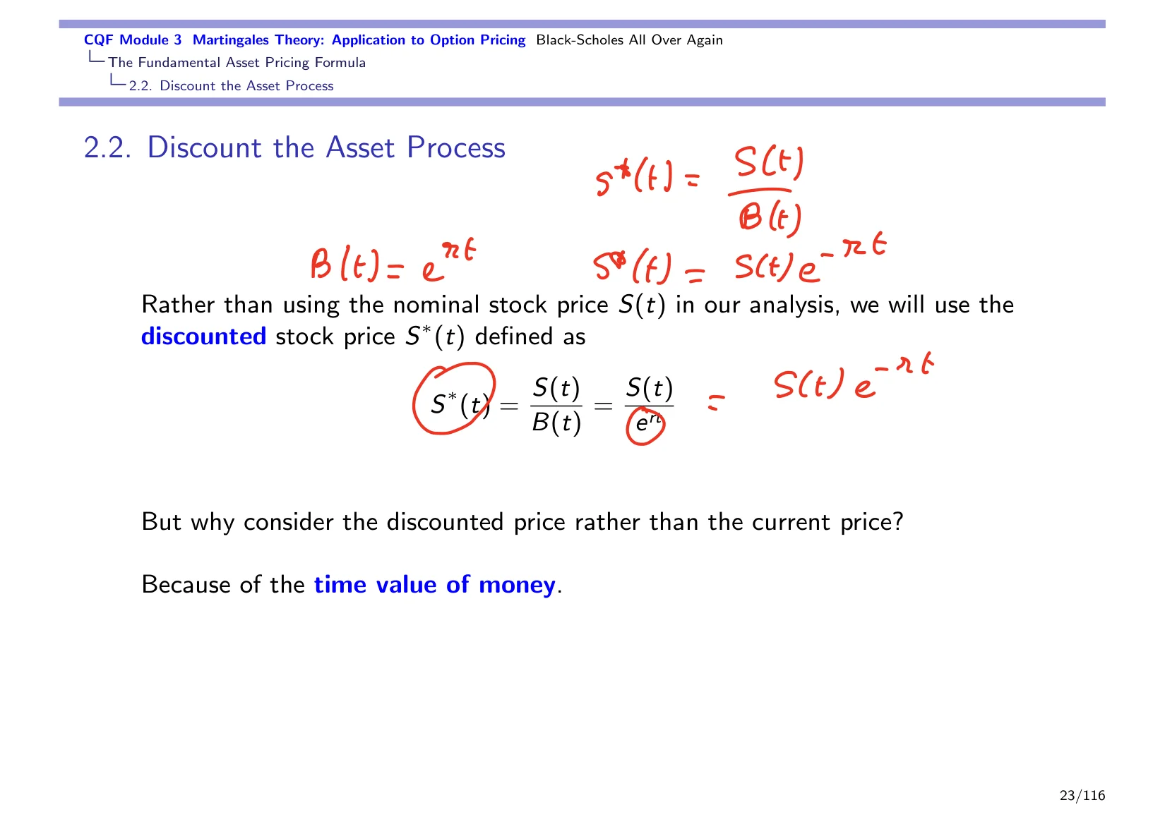
Next, discount the asset price. Discounting the asset price is very simple. We define a new process S*sub*t*. S*sub*t* is just the ratio of the stock price to the price of the risk-free asset. As the price of the risk-free asset B_t is e^(rt), that means that the discounted stock priceDiscounted asset prices Asset prices adjusted for the time value of money by dividing by a discount factor. is S*sub*t* = S_t / e^(rt), which is S_t multiplied by e^(-rt).
That gives us the solution for the value of our discounted stock price. S*sub*t* is simply S*sub*0* multiplied by e^((mu - r - 1/2 sigma^2)t + sigma X_t). S*sub*0* is really just for consistency, because S*sub*0* is S at time zero divided by B at time zero, and B at time zero is one. So it is the same thing as S_0, but for consistency we put a little star there.
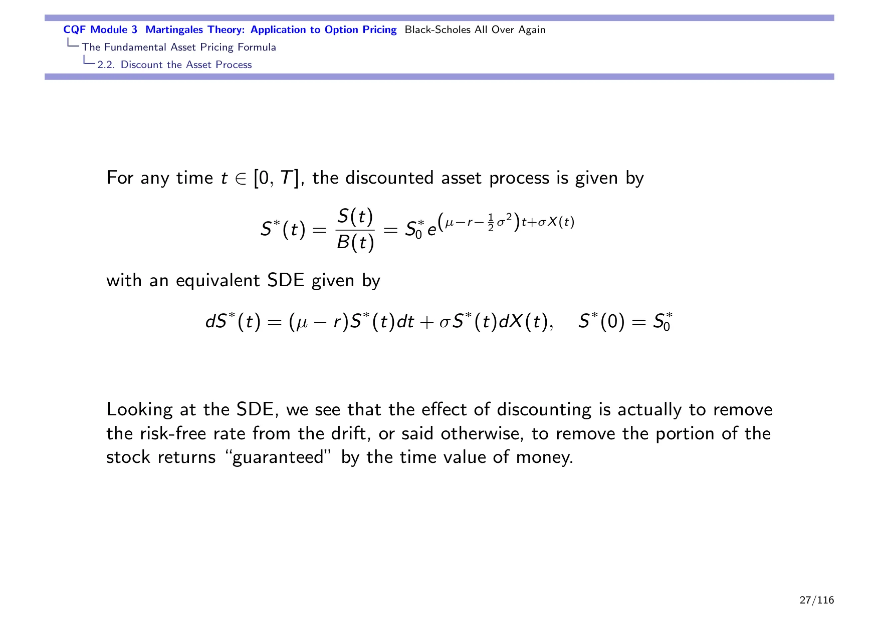
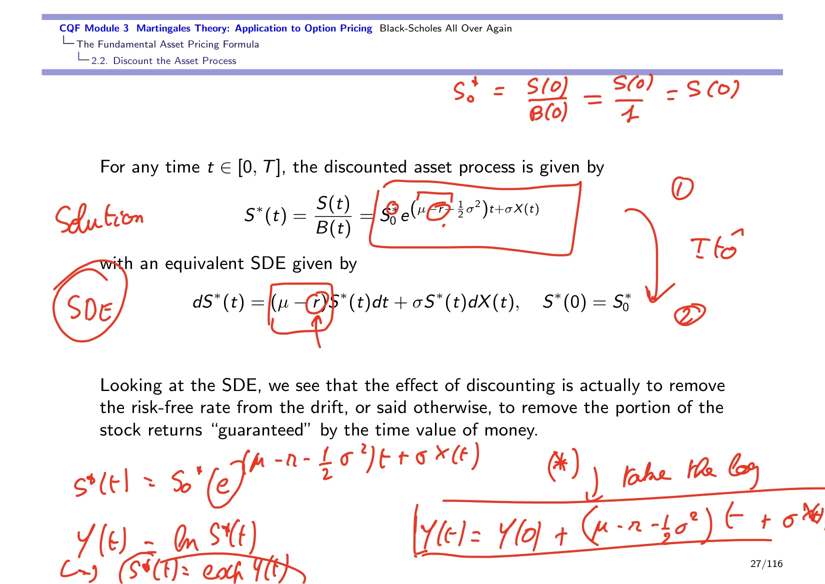
You just take S_t and multiply it by e^(-rt), so that is how you get a minus r. Here you can spot that this looks like a risk premiumRisk premium A risk premium is the excess return required for taking on risk., like an excess return, and that is what it is. Discounting is the same thing as focusing on the excess return and ignoring the short-term rate, the risk-free rate.
When you write the SDE for this dynamics, for this solution, for this stochastic integralStochastic integral A stochastic integral is an integral taken with respect to a stochastic process., the SDE is still geometric. All we do in the drift is remove the risk-free rate from the stock price drift. So this is what happens with the discounted stock price.
To get from the solution to the SDE, there are a couple of ways to do that. The simplest one by now is simply to apply Itô. So you have S*sub*t* = S*sub*0* e^((mu - r - 1/2 sigma^2)t + sigma X_t). Whenever you have an exponential, the first reflex is to get rid of it, so you define a new process Y_t as the log of S*sub*t*.
Taking logs in that equation gives log S*sub*t*, which is Y_t, equal to log S*sub*0*, which is Y_0, plus (mu - r - 1/2 sigma^2)t plus sigma X_t. From there, you can get a stochastic differential equation for Y_t just by taking the differential. Once you have a stochastic differential equation for Y_t, you reverse your transformation.
That is when you apply Itô in order to say: if Y_t is equal to log of S*sub*t*, then S*sub*t* is the exponential of Y_t. You can then apply Itô to the exponential of Y_t given the dynamics of Y_t, which is nice and linear Gaussian. So that is how you get to your stochastic differential equation there.
This is something you have probably seen when you manipulate geometric Brownian motion to solve it and then go from the solution back to the stochastic differential equation. These are the things that you do with Itô. Whenever you have an exponential anywhere, this is the standard trick to try: you take the log.
So now we have a stock price, we have a risk-free rate, and we have a discounted stock price. Now we are ready to look at our change of measure. We are looking at constant currency units, so we remove this natural inflation that we see in finance and economics while dealing with things that already look more stable.
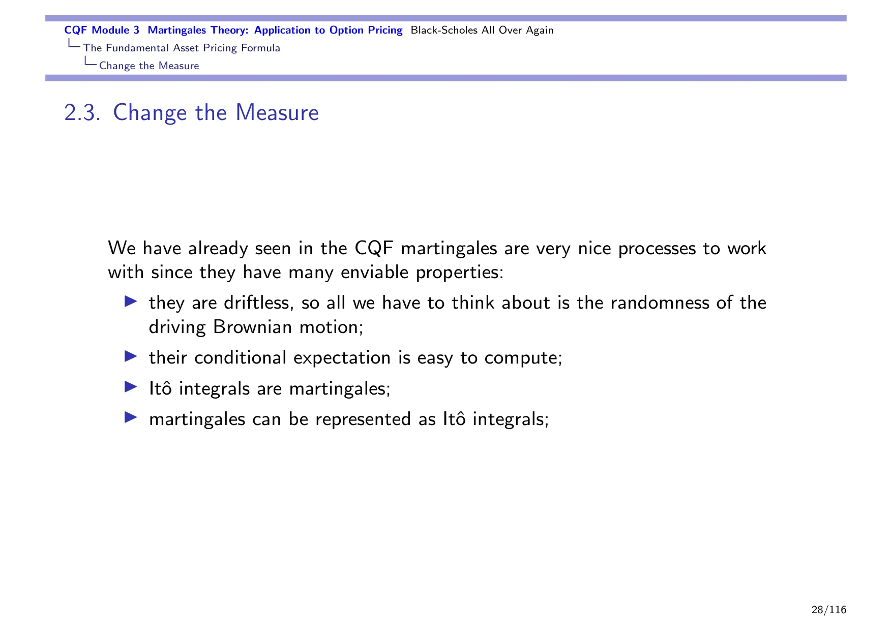
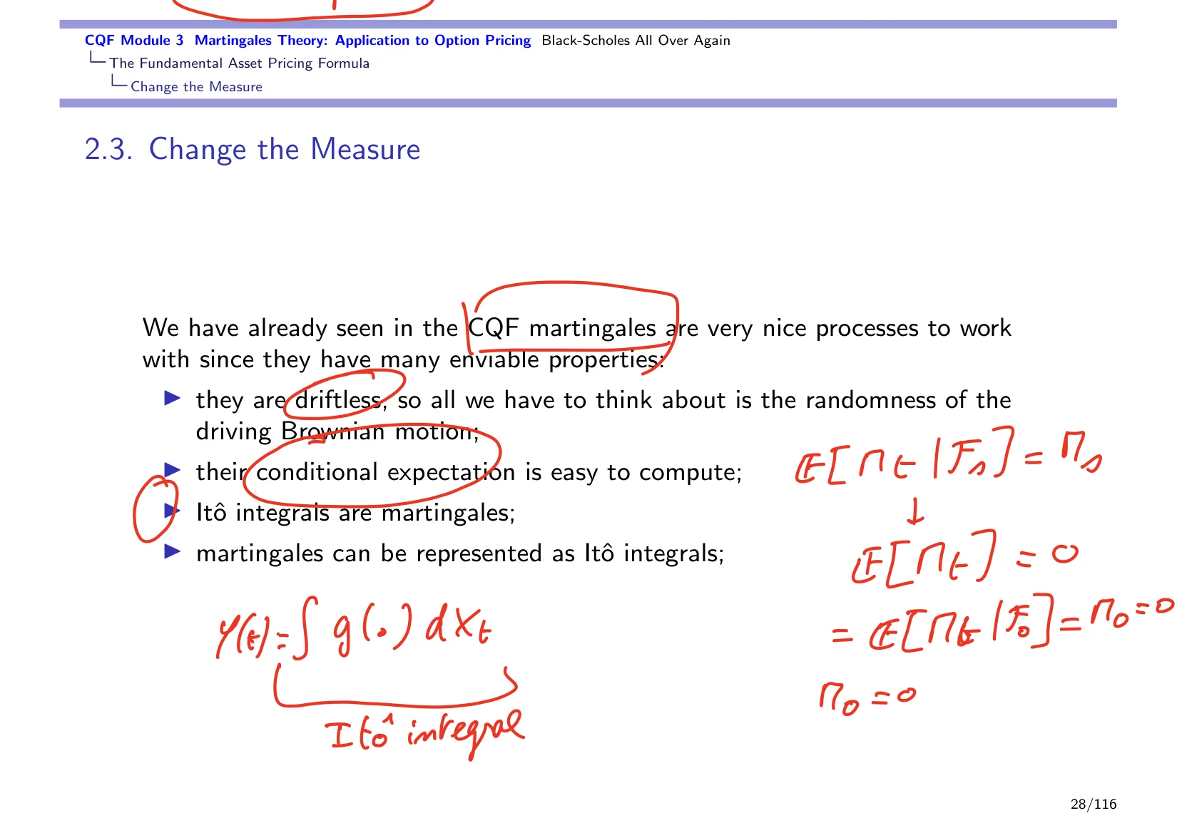
We are going to be ready to transform our problem into one that is entirely probabilistic, where we remove the drift. We have already seen that martingales are nice to work with because they are purely random, meaning that they are driftless. So all you have to think about is the randomness of the driving motion.
We also know that their conditional expectationConditional expectation Conditional expectation is the expected value of a random variable given a specified information set. is easy to compute. Remember, the conditional expectation of some martingale given information up to time little s is just the last known value, which is M_s. And if you take the unconditional expectation of a martingale, it is just M_0. Usually we start it at zero, so M_0 = 0, and that gives you zero.
So martingales are easy to read. If you want them to go away, you just take an expectation. If you want them to stay, they are driftless, they are pure noise. Also, we know that Itô integralsItô integrals Itô integrals are stochastic integrals defined for processes driven by Brownian motion. are martingales, which is very convenient because as soon as we can write the process as an Itô integral, as something that looks like the integral of some function g_t dX_t, we can say that is a martingale.
And we know, since the days of Wiener in the 1920s, that martingales can be represented as Itô integralsItô integrals Itô integrals are stochastic integrals defined for processes driven by Brownian motion.. So whenever you see a martingale, you know that there exists a representation using an Itô integral. These are very nice properties, and that is why we like to work with martingales in probability.
Now the problem so far is that the stock price is not a martingale, and even the discounted asset price, S*sub*t*, is not generally a martingale under the measure P in the real world. To see that, think about its dynamics: dS*sub*t* = (mu - r) S*sub*t* dt + sigma S*sub*t* dX_t. We know that stocks are risky, they have a diffusion. If they are risky, they should return something greater than the risk-free rate, so mu should be greater than r.
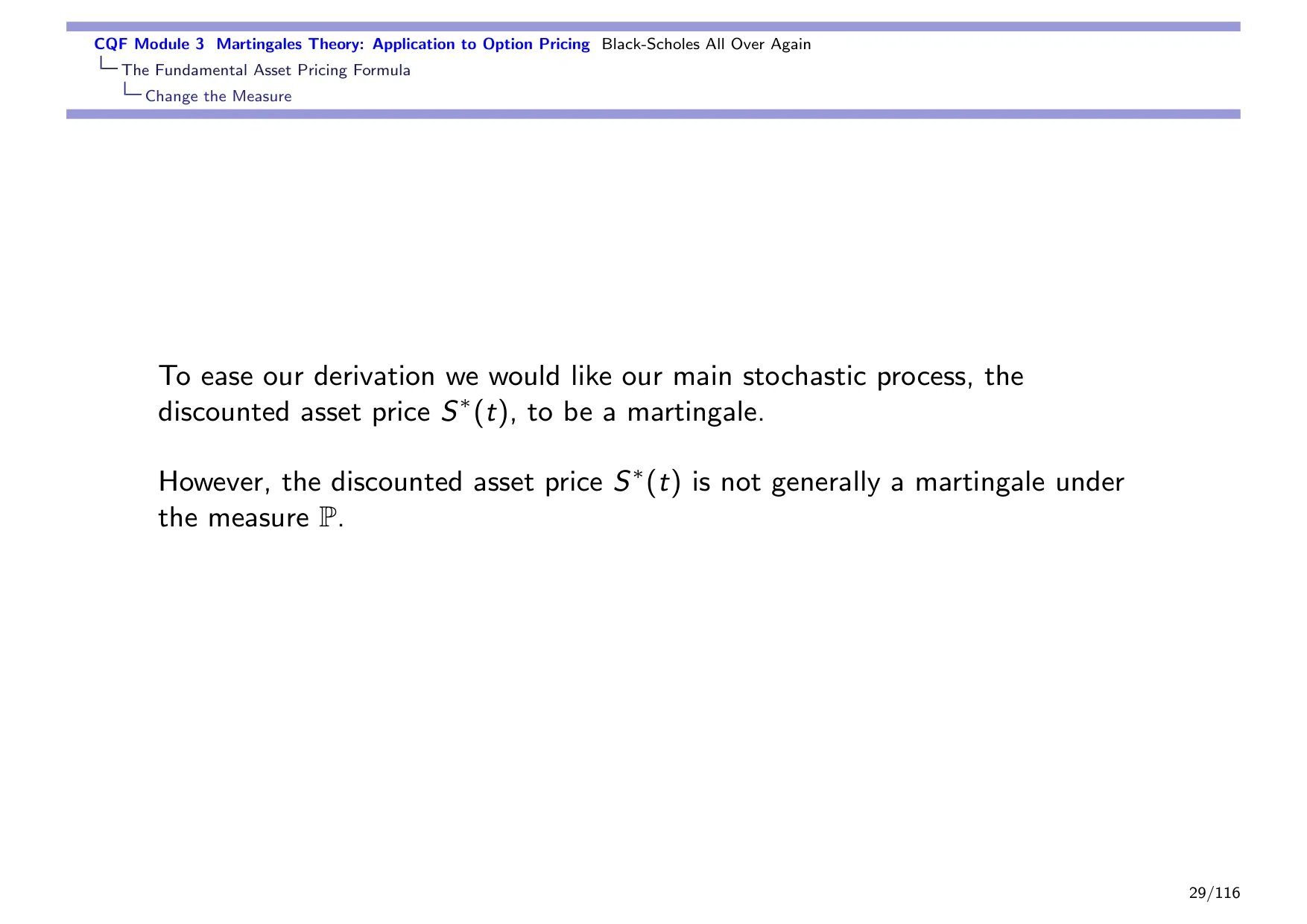
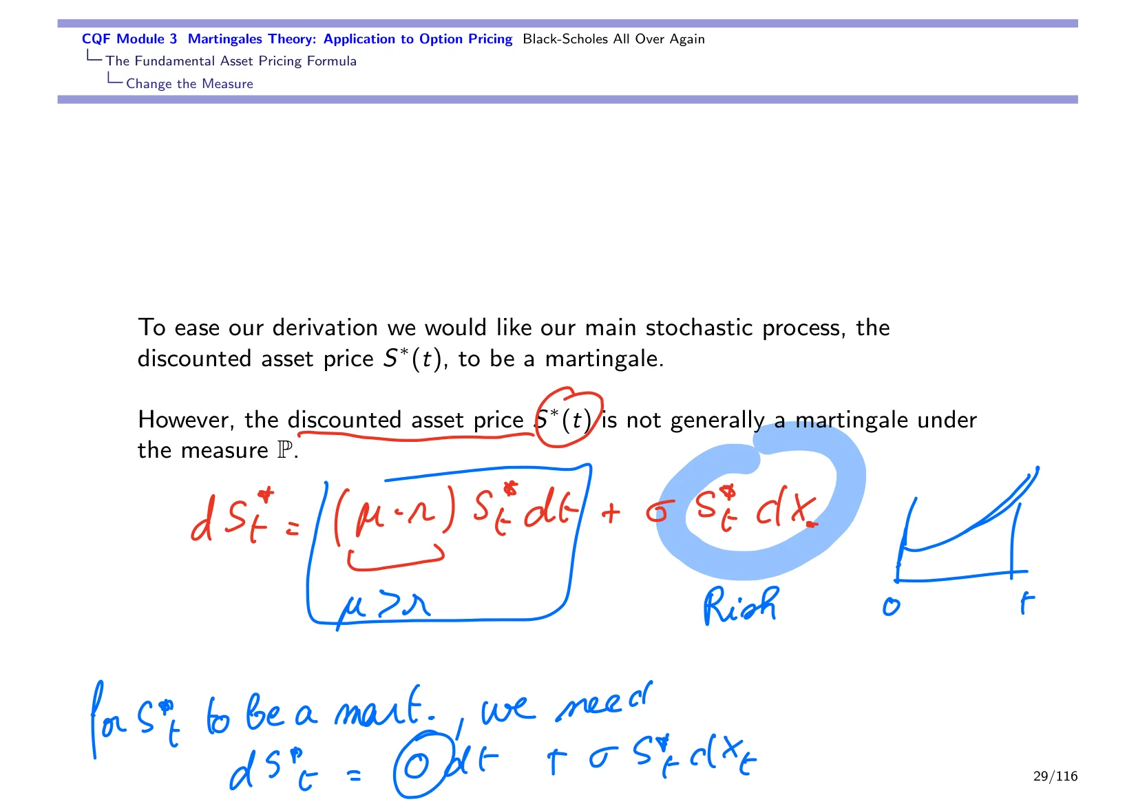
If mu is greater than r, this is not equal to zero by definition. For S*sub*t* to be a martingale, we would need it to be driftless, meaning that in its stochastic differential equation the drift term is zero. So we would need to write dS*sub*t* = 0 dt + sigma S*sub*t* dX_t. Of course, this only happens if mu = r.
But in the real world, we should not have mu = r. Stocks are risky, so we need to be compensated for the risk that we take. Therefore mu should be greater than r. Over time, stock prices, even discounted stock prices, should rise because we should be compensated for taking risk over a longer period of time.
So stock prices, even discounted stock prices, are not martingales; they are actually submartingalesSubmartingales Submartingales are processes whose conditional expected future value is at least their current value.. That is why we need to change measure, because we need to find a way to convert our stock price into a martingale so that we can make our calculations a bit easier. We want to focus only on the diffusion and not care about the drift.
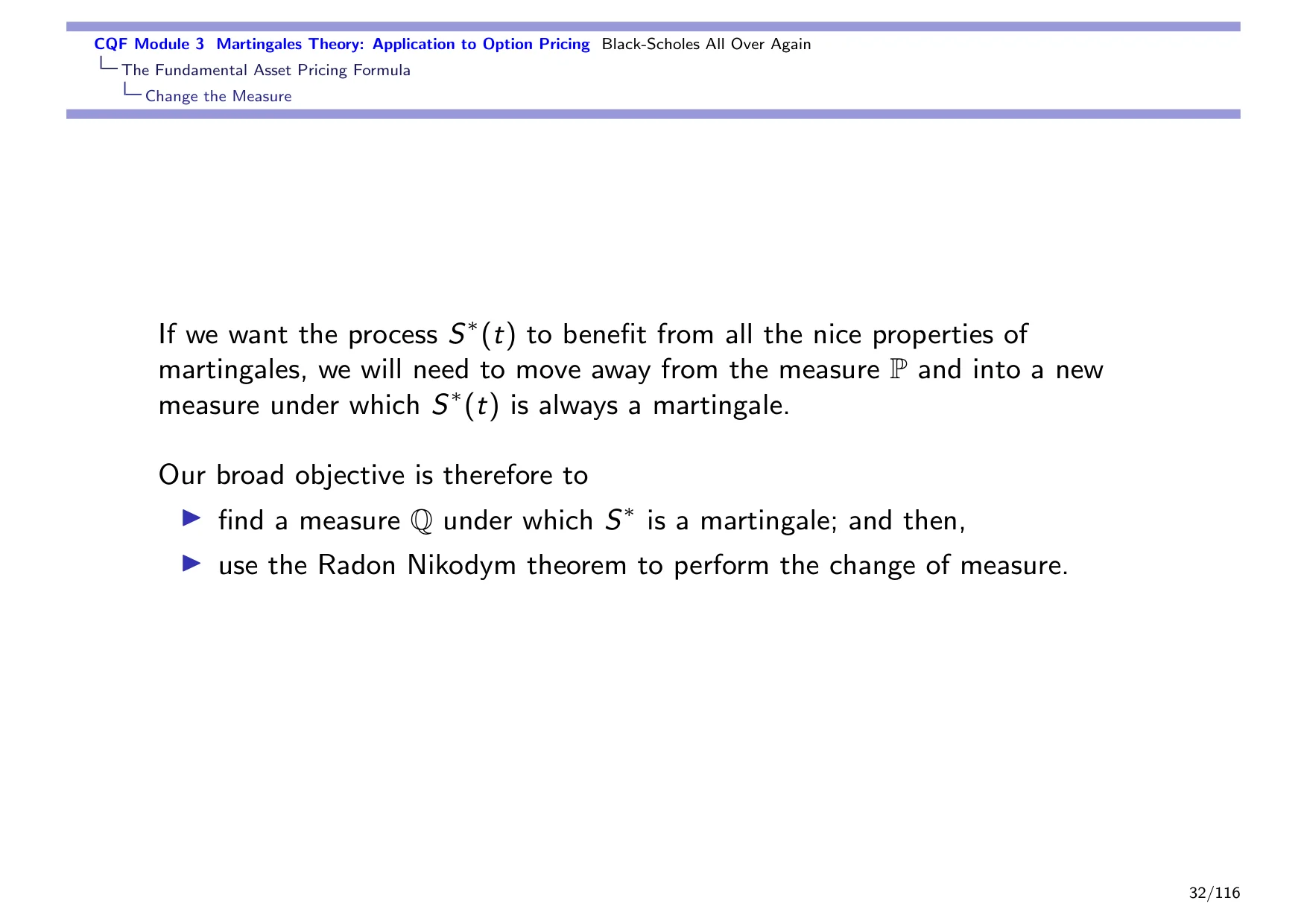
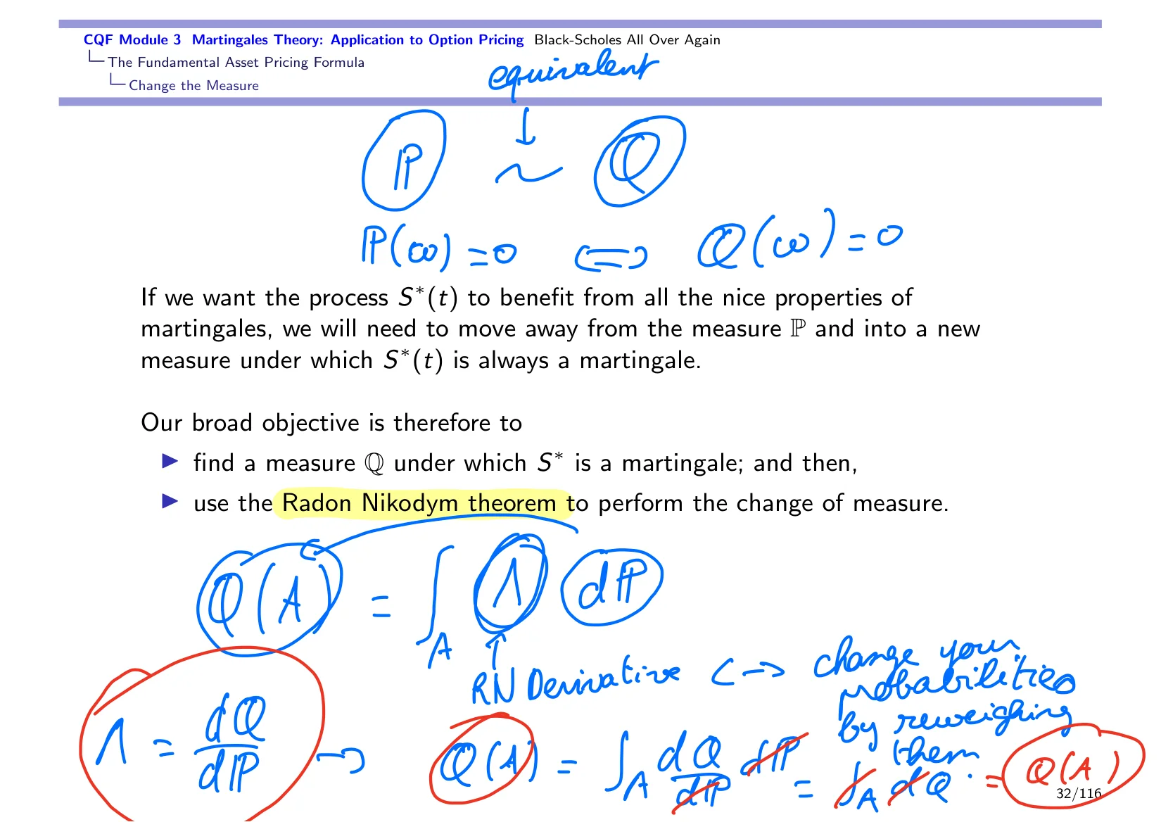
To do that, we have a powerful result in probability theory called the Radon-Nikodym theoremRadon-Nikodym theorem The Radon-Nikodym theorem gives conditions under which one measure has a derivative, or density, relative to another.. The Radon-Nikodym theorem tells you: let us take a measure P, a probability distribution for outcomes, and let us take an equivalent probability distribution Q.
What Radon-Nikodym means when they say equivalent is actually quite simple. It does not mean that events need to have the same probability, but events that are impossible under probability distribution P should remain impossible under probability distribution Q. Think about it: we are in a physical world where elephants, fortunately, do not fly. The probability that elephants fly is zero.
So we are going to look for equivalent probability measures, meaning distributions of probabilities in alternate realities, the multiverse or whatnot, where elephants do not fly either.
If the probability of an event \(\omega\) is zero with probability distribution \(P\), then the probability of the same event \(\omega\) should also be zero with probability distribution \(Q\). Elephants cannot fly here; they should not fly there. That is all we require in order to have two measures that are equivalent.
After that, the probability that things happen might be different, but the probability of something that is impossible remains zero regardless of where we are. Now, what the Radon-Nikodym theoremRadon-Nikodym theorem The Radon-Nikodym theorem gives conditions under which one measure has a derivative, or density, relative to another. tells you is that if you want to go from \(P\) to \(Q\), if you want to convert a probability with distribution \(P\) into a probability with distribution \(Q\), you are going to apply this formula. The probability of an event, say \(A\), with probability measure \(Q\), is the integral of something called the Radon-Nikodym derivativeRadon-Nikodym derivative The Radon-Nikodym derivative is the density that converts one probability measure into another by reweighting probabilities. times \(dP\).
So you reweight. This is a way to change the weight inside your probabilities so that the distribution \(P\) looks more and more like the distribution \(Q\). You tweak your probabilities by adding a little bit more weight so that an event that had, for example, one-sixth probability under \(P\) would now have two-sixths probability, or one-third, under \(Q\). So all this Radon-Nikodym derivativeRadon-Nikodym derivative The Radon-Nikodym derivative is the density that converts one probability measure into another by reweighting probabilities. does is change the probabilities by reweighting them.
And that is where this idea that we needed equivalent probability measures is important, because if something has probability zero, no matter the weight that you put, the probability still stays zero. Now it turns out that the Radon-Nikodym derivative, \(\lambda\), is simply, drum roll, \(dQ/dP\). It is the ratio of likelihoods. It is the ratio of your probability \(Q\) divided by your probability \(P\).
And yes, it does make sense, because that means that \(Q(A)\) is equal to the integral over \(A\) of \(dQ/dP\) multiplied by \(dP\). So what you do is cancel the \(P\)'s, leaving you with the integral over your event \(A\) of \(dQ\). Of course, the integral kills the differential. We already used the reverse rule earlier, which gives you simply \(Q(A)\). So yes, \(Q(A) = Q(A)\), that is genius. One is equal to one, beautiful.
But what this says is that, really, when you look at your Radon-Nikodym derivative and your Radon-Nikodym theorem, which is a purely abstract result, the way to change the weight is simply by looking at the ratio of how likely something is under one probability versus how likely it is under another. Somebody mentioned earlier on that importance samplingImportance sampling Importance sampling is a Monte Carlo technique that improves estimation by drawing samples from a more convenient distribution and adjusting the weights. is a very important technique, no pun intended, in statistics, and you also find it applied in reinforcement learning. It helps you sample from one distribution and then adjust the probabilities based on another distribution, which is a very powerful technique. It is just that: a change of measure.
Now, this in fact is not usable for us right now, because we would like to have a result that helps us change probability measure more at the level of our stochastic processes, more at the level of our Brownian motion. We do not want a big result that tells us \(Q(A) = Q(A)\). So what are we going to do? We are going to use a result that is called Girsanov's theorem, and Girsanov's theorem works beautifully. Girsanov's theorem is actually a corollary of Radon-Nikodym applied to stochastic processes, especially to diffusion processesDiffusion processes Stochastic processes whose evolution includes a continuous random diffusion term..
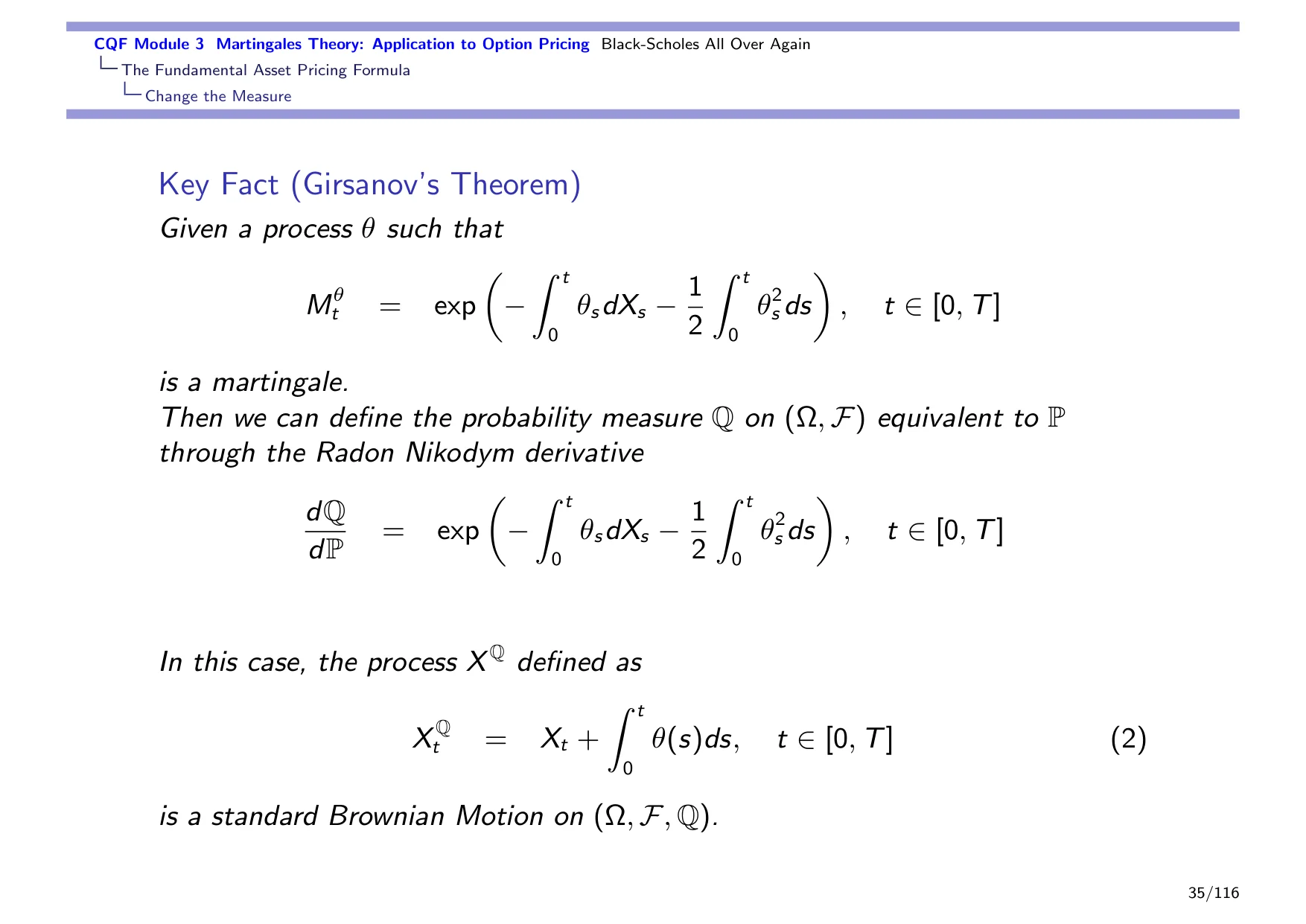
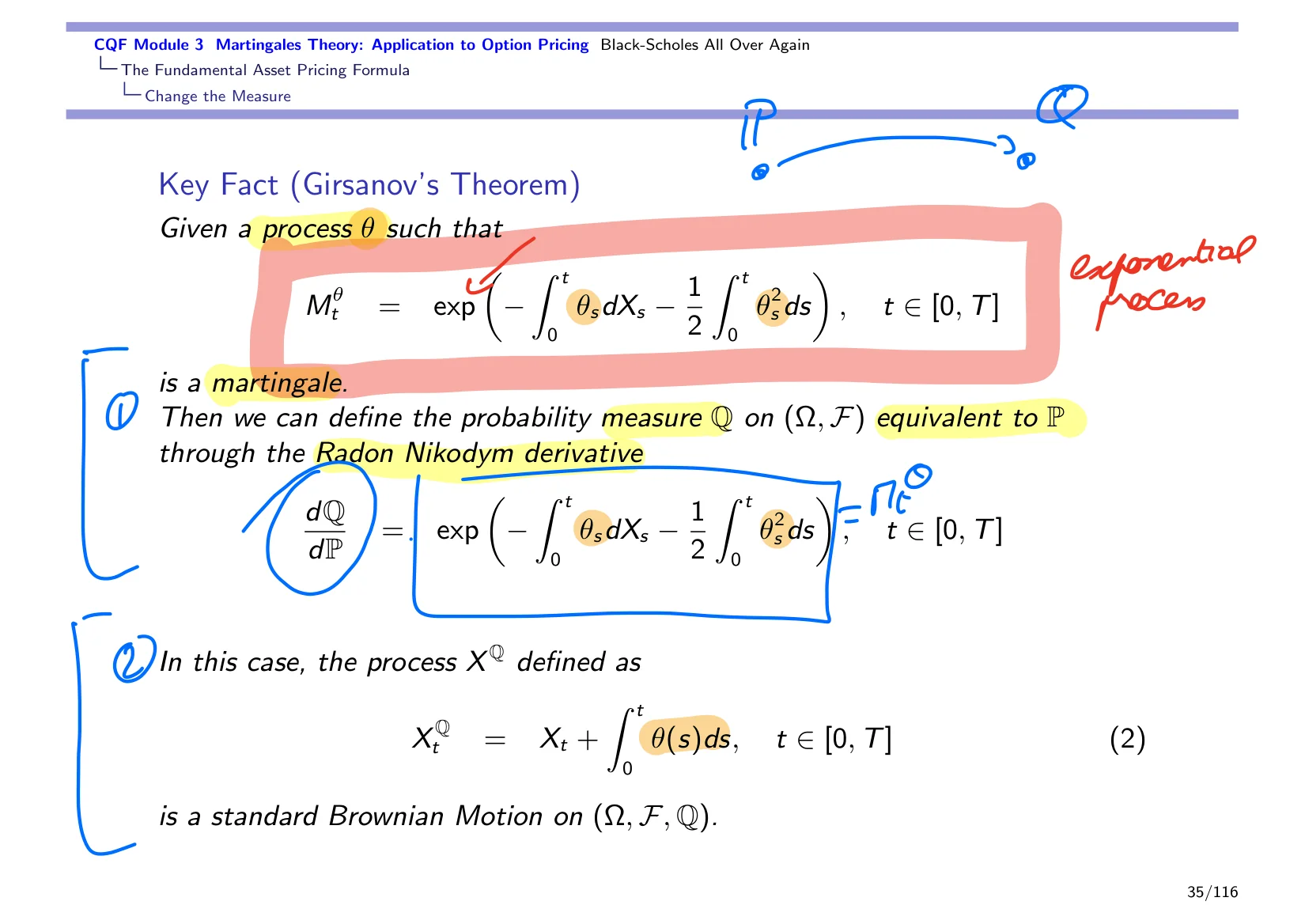
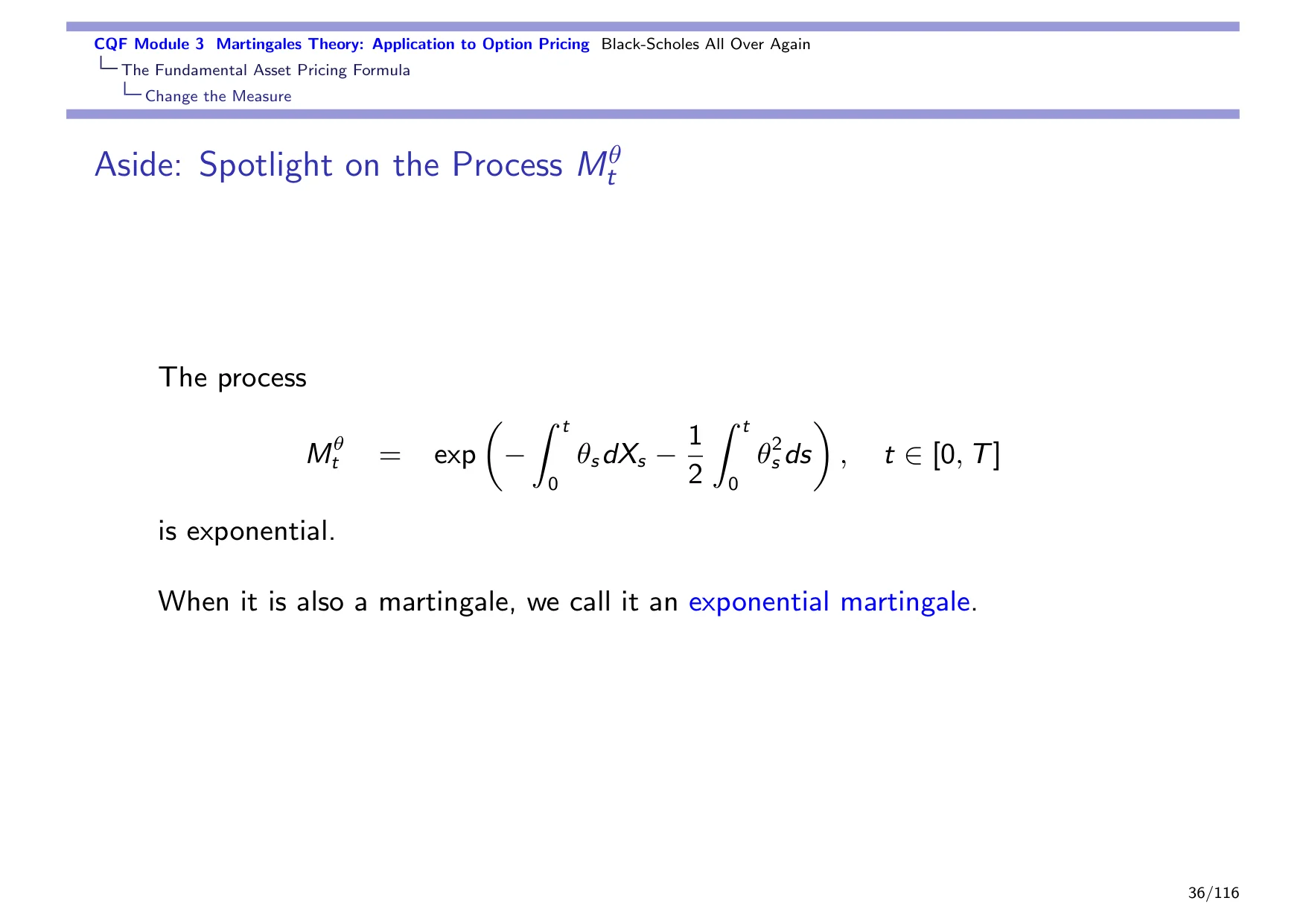
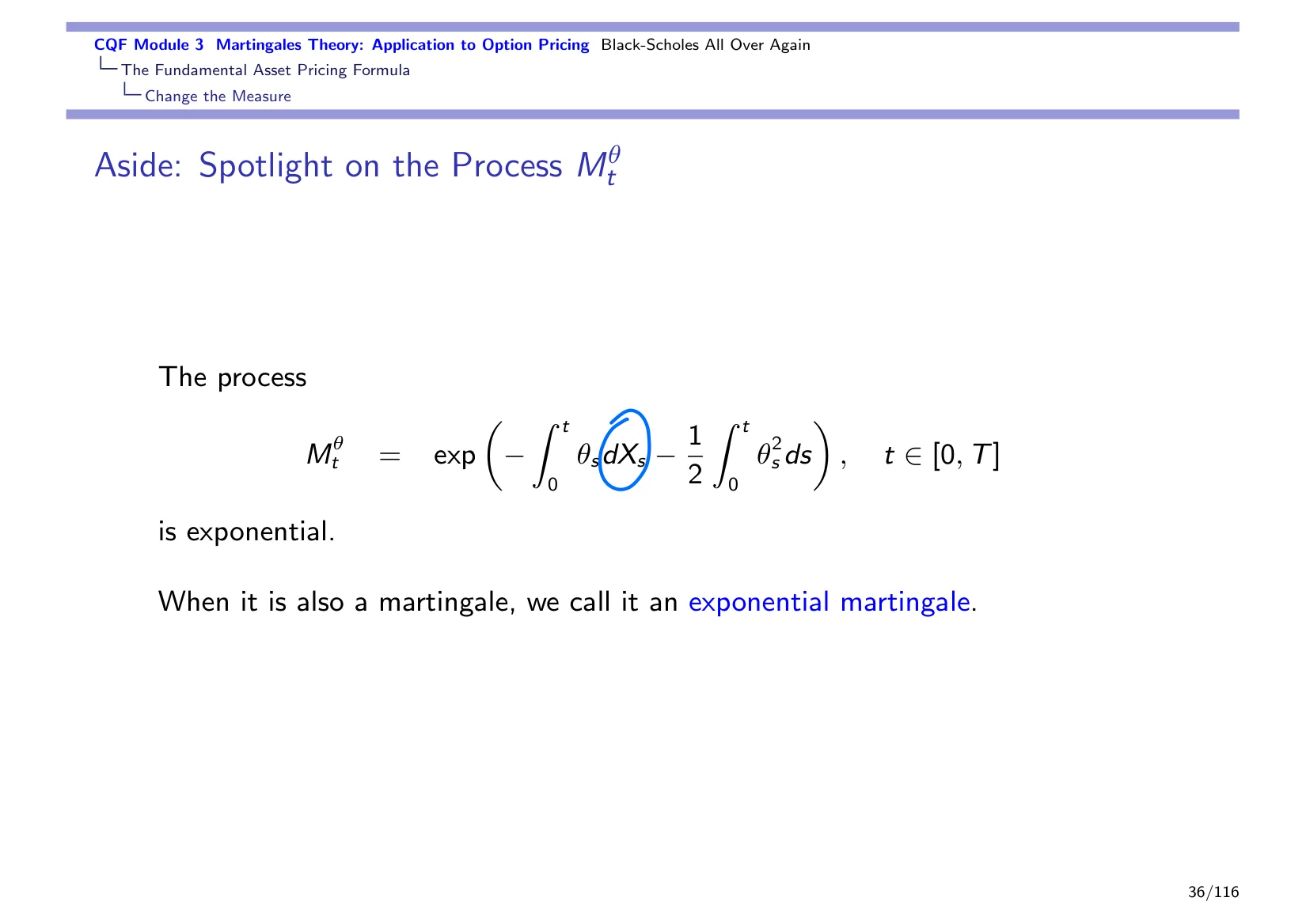
Now, you have to start somewhere, and our starting point is this: we start with some process \(\theta\)Theta process / process \(\theta\) A process denoted by theta, often used for a trading strategy or coefficient in a stochastic integral. such that this exponential process, and yes, it is an exponential process, \(M_t\) parameterized by \(\theta\), which is the exponential of minus the integral from zero to \(t\) of \(\theta_s\, dX_s\), minus one-half the integral from zero to \(t\) of \(\theta_s^2\, ds\), is a martingale. So if we have a process \(\theta\), and using this process \(\theta\) we can construct an exponential process that is also a martingale, called more succinctly an exponential martingale, then we can use that to define a new probability measure \(Q\) on \((\Omega, \mathcal{F})\).
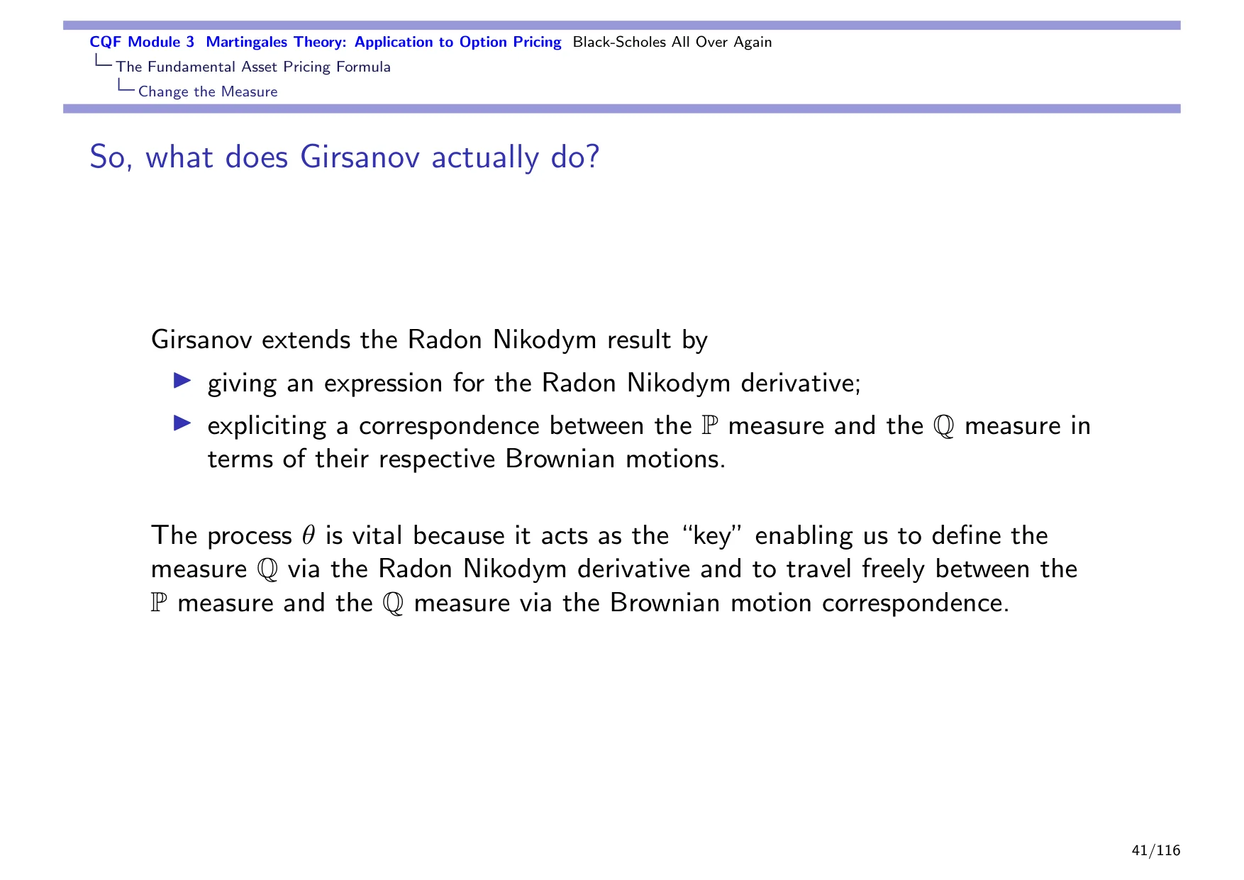
This measure is going to be equivalent to \(P\), which is exactly what we want, and that is exactly what Radon-Nikodym requires. The nice thing is that we know exactly what the Radon-Nikodym derivative is, because the Radon-Nikodym derivative, so \(dQ/dP\), the ratio of likelihoods, is simply the exponential martingale itself. It is simply \(M_t^{\theta}\). So an exponential martingale is something that we can use as a Radon-Nikodym derivative to go from planet \(P\), or from probability distribution \(P\), to probability distribution \(Q\).
So this gives us already the Radon-Nikodym derivative, but there is another element, element two in Girsanov, which tells us: okay, so what we have done so far is we started here on some planet \(P\), with its own Brownian motion \(X_t\), and we have been able to define a planet \(Q\). We know that to go from \(P\) to \(Q\), just take the Radon-Nikodym derivative train, \(dQ/dP\), which is defined via some exponential martingale, and of course we could go from \(Q\) to \(P\) the other way around via \(dP/dQ\). It is not a one-way trip; we go one way, we come back the other.
Now, what Girsanov also tells us is this: under \(Q\), \(Q\) has its own Brownian motion, let us call it \(X_t^Q\), and now we are going to get \(X_t\) under \(P\) and \(X_t^Q\) to shake hands somewhere in the middle by finding a way to express one in terms of the other. That is point two. Point two tells us that now that we have established \(P\) and \(Q\), and a bridge between the two, I can tell you that a unit of randomness, which is called a Brownian motion under \(P\), has a cousin, a distant relative on \(Q\), which is also a Brownian motion under \(Q\).
But there is a slight tweak, because the Brownian motion under \(Q\), \(X_t^Q\), is actually the Brownian motion under \(P\) plus some drift, and this drift depends on our good old friend, or good new friend, \(\theta_s\). So you see that this process \(\theta\)Theta process / process \(\theta\) A process denoted by theta, often used for a trading strategy or coefficient in a stochastic integral. plays a key role: find the process \(\theta\), define an exponential martingale, with this exponential martingale you can get a Radon-Nikodym derivative, which acts as a shuttle between probability \(P\) and probability \(Q\), and still with this process \(\theta\), you can define the meaning of a Brownian motion under \(Q\) in terms of the meaning of a Brownian motion under \(P\).
So for us, of course, what we are going to be interested in is to take \(P\) as the real world, where you do your trading, your portfolio management, your risk management, your shopping, and basically where you live. And in order to price an option, we are going to create a new world, a new probability system, just to make it easy for us to calculate stuff. We only go there to calculate stuff, and then we bring back the calculation that we make.
And that is, let us call it, planet finance, with a big dollar sign on it, and a few pound signs there, and euros and yen, etc. That is planet finance, and we only go there to price stuff. Because in planet finance, what we want is to find a probability system such that our discounted stock price is a martingale. And that is going to make our calculations easier.
So it is just a computational trick, nothing more.
Based on the characteristics that we want to see, based on what makes our calculations easier, we still live in the real world. I don't know about you, but I try to live in the real world. We only go to the other thing because it's a convenient framework to price stuff, and then we bring back the price here. And that's all there is to it. Turning things upside down is really just a matter of, purely, a computational trick. It's a computational trick that's a bit heavy, because we manipulate entire probability distributions, so the probabilities change. But again, probabilities are just a mathematical tool themselves. Don't get attached to them; it's just a bunch of variables and weights, and that's it. So that's what we do.
Now, what we're going to do, just five minutes before the break. I can recommend some books. Not all of them are readable. Do I have some? Oh, no. I always say that I wanted to add them. I'll collect a few books and send Melody or Rita a list. I have that on, actually, another lecture that I used to do a long time ago. I always think I need to put that here, and I always forget. There are a few books; however, not all of the books are readable. That's one of the problems with this topic. You're getting into stuff that's a bit technical, in case you didn't notice, in case you missed the last hour and a half while getting into technical stuff. Warning.
Now, the process density, there is a little spotlight; I'll let you go through it. The process density is an exponential martingale. There are several ways to check whether a process is an exponential martingale. We're not going to have to worry too much about that tonight because our processes are going to be very nice. The thetas that we deal with are all constant, in which case we know that this process, we can show that this process, is a martingale. So, yes, I spotted the little typo that I've had for now probably a year. It's fixed here. And so there are two conditions that you can check in order to make sure that you've got an exponential martingale.
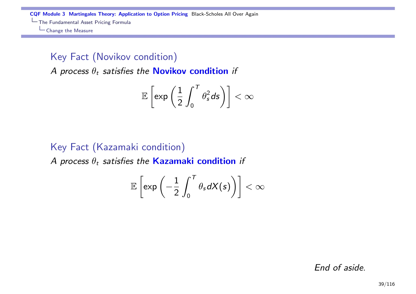
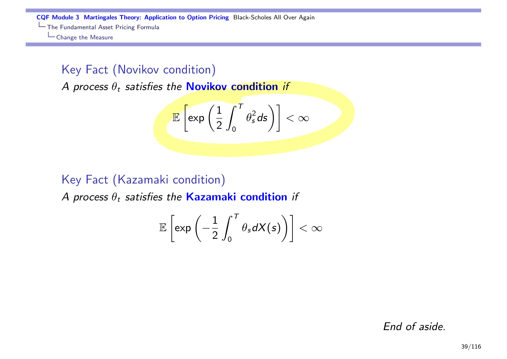
One is by NovikovNovikov / Novikov condition A condition used in stochastic calculus to justify certain measure changes and exponential martingales., the other is by Kazamaki. This one is usually the most useful because Kazamaki shows up at times; I've used it a couple of times, but predominantly what you're going to mostly use is the Novikov condition in order to make sure that the process that you've got is a martingale. Now, the other side is that Girsanov has changed measures beyond Black-Scholes. We use that, of course, to price all types of derivatives, equity optionsEquity options Options written on equities such as stocks or equity indices., interest rates, credit and securities, but we also use that in portfolio selection for risk-sensitive investment management problems, and yes, it's used in importance sampling techniques in Monte Carlo-based methods for reinforcement learning. Thank you.
arbitrage opportunity
Arbitrage is a trading strategy that yields a sure profit without requiring an initial investment or exposing the trader to risk.
Arbitrage is a self-financing strategy that produces a positive payoff in some states and never a negative payoff, typically with zero initial cost. It is a key no-arbitrage concept in finance.
No-arbitrage conditions are central to pricing theory because they rule out inconsistent prices. Many pricing formulas, including those in this lecture, are derived by excluding arbitrage.
The lecture uses arbitrage as the motivating condition behind the pricing setup and as the reason for introducing measure change. Carry trades are mentioned as an example of an arbitrage-like idea.
score: 22 · inline: first_in_lecture
The binomial model is a discrete-time model where an asset price moves up or down by fixed factors over successive steps.
The binomial model represents price evolution on a tree with two possible moves at each time step. It is a simple discrete framework for option pricing and hedging.
It provides an intuitive starting point for understanding no-arbitrage pricing and replication. In many courses, it serves as the discrete precursor to continuous-time models.
The lecture refers to the binomial model as the starting point from which the Black-Scholes result can be motivated. It is used as a comparison point for the continuous-time derivation.
score: 18 · inline: first_in_lecture
Black-Scholes is the standard continuous-time framework for pricing options and related derivatives.
Black-Scholes is a foundational option-pricing framework built on a stochastic model for the underlying asset and a no-arbitrage pricing principle. It leads to both a pricing PDE and a closed-form formula in the standard case.
It is one of the central results in mathematical finance and a benchmark for derivative pricing. Understanding it helps connect stochastic processes, PDEs, and pricing theory.
The lecture presents the Black-Scholes setting as the main target of the derivation and repeatedly refers to the formula and equation that arise from it. It is the anchor topic for the measure-change argument.
score: 18 · inline: first_in_lecture
Black-Scholes PDE
The Black-Scholes equation is the PDE that the option price satisfies in the standard Black-Scholes model.
The Black-Scholes equation is a partial differential equation for the value of a derivative as a function of time and the underlying asset price. It encodes the no-arbitrage dynamics of the standard model.
It is one of the main mathematical forms of the Black-Scholes pricing result. Solving it gives the option value in the continuous-time framework.
The lecture treats the Black-Scholes PDE as an intermediate result on the way to the final pricing formula. It is presented as the equation that emerges from the model assumptions and hedging argument.
score: 20 · inline: first_in_lecture
The Black-Scholes formula is the closed-form expression for the price of a standard European option in the Black-Scholes model.
The Black-Scholes formula gives an explicit price for a European-style option under the standard assumptions of the Black-Scholes model. It is the closed-form counterpart to the Black-Scholes equation.
It is a landmark result because it turns a pricing problem into a direct computation. The formula is widely used as a benchmark in derivatives pricing.
The lecture repeatedly points toward the formula as the final goal of the derivation. The earlier measure-change and PDE steps are presented as routes to reach it.
score: 18 · inline: first_in_lecture
The bond price is the current value of a bond in the market.
The bond price is the amount paid today to buy a bond or the value assigned to it in the market. In pricing models, it often serves as a numeraire or discounting reference.
Bond prices are central to discounting future cash flows and comparing assets on a present-value basis. They also appear in hedging and measure-change arguments.
The lecture uses the bond price as part of the notation in the pricing setup. It appears as a basic market quantity alongside the risky asset and the Brownian motion.
score: 11 · inline: first_in_lecture
Brownian motion under \(Q\)
Brownian motion is a continuous-time stochastic process with independent, normally distributed increments.
Brownian motion is a fundamental random process used to model continuous random fluctuations. It has continuous paths and stationary independent increments.
It is the basic noise source in many stochastic models, including option pricing. Changing the measure often changes the drift while preserving the Brownian structure.
The lecture discusses Brownian motion both in the original model and under the new measure. It is part of the stochastic dynamics that the measure-change argument modifies.
score: 19 · inline: first_in_lecture
Call option, call
A call option is a derivative that gives the right, but not the obligation, to buy an asset at a fixed strike price.
A call option is a contract whose payoff depends on the asset price being above the strike at expiration. Its value reflects the chance of ending in the money.
Call options are a standard example in derivative pricing and hedging. They are often used to illustrate the Black-Scholes framework.
The lecture uses a call option as the motivating payoff to be priced. It appears in the discussion of how the model and measure change lead to the final pricing result.
score: 12 · inline: first_in_lecture
Call payoff, max of ST minus E or zero
A call payoff is max(ST − E, 0), the amount paid by a call option at maturity.
The call payoff is the terminal value of a call option. It equals the positive part of the stock price at maturity minus the strike price, written as max(ST − E, 0).
It is the basic payoff used to price and hedge call options. Understanding the payoff is the starting point for deriving the option value.
The lecture introduces the call payoff explicitly when discussing option pricing at maturity. It is one of the two standard payoffs used in the Black-Scholes setup.
score: 20 · inline: first_in_lecture
carry trades
A carry trade is a strategy that seeks profit from differences in funding and investment returns.
A carry trade is a position that borrows in one asset or currency and invests in another with a higher expected return. In idealized discussions, it is often treated as an arbitrage-like strategy.
It is a useful example when discussing arbitrage and funding effects in finance. It helps connect abstract pricing ideas to market practice.
The lecture mentions carry trades as an example of arbitrage in the broader discussion of no-arbitrage pricing. It serves as a concrete market illustration rather than a main derivation step.
score: 13 · inline: first_in_lecture
future cash flows, intermediate cash flow
Cash flows are the payments or receipts generated by an asset or contract over time.
Cash flows are the amounts of money paid or received at different times. In valuation, they are the basis for present-value calculations.
Pricing often reduces to discounting expected future cash flows under an appropriate measure. Understanding the timing of cash flows is essential for derivative valuation.
The lecture refers to future cash flows and notes when intermediate cash flows are absent. This supports the move from payoff description to pricing under the chosen measure.
score: 12 · inline: first_in_lecture
changes of measure, reweighting
A change of measure is a transformation that replaces one probability measure with another, usually by reweighting probabilities.
A change of measure is a method for rewriting probabilities and expectations under a new measure. It is typically implemented using a Radon-Nikodym derivative.
It is a central technique in stochastic calculus and mathematical finance because it can simplify drift terms and pricing calculations. Many no-arbitrage arguments rely on it.
The lecture presents change of measure as the main mechanism behind the derivation and repeatedly describes it as reweighting probabilities. It is tied directly to the Radon-Nikodym derivative and the exponential martingale.
score: 22 · inline: first_in_lecture
A change of numeraire is a pricing method that switches the reference asset used to measure values.
A numeraire is the asset used as the unit of account, and changing the numeraire means expressing prices relative to a different reference asset. This often comes with a corresponding change of probability measure.
It can simplify pricing formulas and make certain assets or payoffs easier to analyze. It is a standard technique in advanced derivative pricing.
The lecture mentions change of numeraire as part of the broader pricing toolkit. It appears alongside the numeraire technique as a way to reframe the valuation problem.
score: 16 · inline: first_in_lecture
Conditional expectation is the expected value of a random variable given a specified information set.
Conditional expectation is the average value of a random variable after conditioning on known information. In stochastic processes, it is often taken with respect to a filtration or a past time.
It is the basic tool for pricing, martingales, and dynamic models because it formalizes prediction from available information. Many results in the lecture are expressed through conditional expectations.
The lecture uses conditional expectation in the discussion of martingales, describing it as the last known value in the relevant filtration. This supports the intuition behind the process density argument.
score: 16 · inline: first_in_lecture
A contingent claim is a derivative contract whose payoff depends on future market outcomes.
A contingent claim is a financial claim with a payoff that depends on the realization of some future event or asset price. Options are a common example.
Contingent claims are the main objects priced in derivative theory. They are the reason tools like no-arbitrage and measure change are introduced.
The lecture uses the term as another name for the derivative being priced in the Black-Scholes setting. It appears when the payoff is being described in general terms.
score: 16 · inline: first_in_lecture
Continuous time is a modeling setting where variables evolve at every instant rather than at separate time points.
Continuous time models describe evolution over an unbroken time axis, allowing calculus and stochastic differential equations to be used. This contrasts with discrete-time models such as binomial trees.
It is the natural setting for the Black-Scholes framework and many stochastic calculus methods. It allows the lecture to move from discrete intuition to continuous pricing.
The lecture explicitly states that the model is in continuous time before introducing the stochastic and measure-change machinery. This sets the stage for Brownian motion and the Black-Scholes PDE.
score: 10 · inline: first_in_lecture
Deflate prices, deflate our prices
To deflate prices means to divide prices by a reference asset or discount factor to simplify valuation.
Deflating prices means rescaling asset values by a chosen numeraire or discount factor. This produces a transformed price process that is easier to analyze.
Deflation is a standard step in pricing arguments because it can turn a discounted price into a martingale under the right measure. That property is central to no-arbitrage valuation.
The lecture uses the phrase when introducing the transformation needed for the measure-change argument. It is part of the setup that leads to the process density and equivalent measure.
score: 12 · inline: first_in_lecture
Delta is a sensitivity measure, usually the derivative of an option price with respect to the underlying asset price.
Delta measures how a derivative’s value changes when the underlying asset price changes. In hedging, it is often interpreted as the number of shares needed to offset small price moves.
It is one of the most important risk sensitivities in option pricing and hedging. It connects the PDE view of pricing with the trading strategy view.
The lecture refers to delta both as a hedge ratio and as the derivative coming from the PDE. It is used when discussing how many shares to hold in the replicating portfolio.
score: 13 · inline: first_in_lecture
price of a derivative as an expectation
The values assigned to derivative contracts, often computed as an expected discounted payoff.
Derivative prices are the market values of contracts whose payoff depends on an underlying asset or state variable. In this lecture, they are presented as quantities that can be computed as expectations.
Pricing derivatives is the main goal of the lecture, and the expectation form connects stochastic modeling with valuation. It also links the model for asset dynamics to the contract value.
The lecture uses derivative prices as the target quantity to generate and compute, including the idea of pricing a derivative as an expectation. This frames the later martingale and discounting arguments.
score: 21 · inline: first_in_lecture
Financial instruments whose value depends on the performance of another asset or variable.
Derivatives are contracts whose payoff is determined by an underlying quantity such as a stock price, interest rate, or index. Their value is derived from that underlying rather than fixed in advance.
They are the main objects being valued in this lecture, so understanding them is essential for the pricing framework. The course uses them to motivate expectation-based valuation methods.
The lecture refers to valuing and pricing all types of derivatives, using the term in a broad financial sense. It serves as the central application for the stochastic pricing setup.
score: 11 · inline: first_in_lecture
Interest rates that are assumed to be known in advance and not random.
Deterministic interest rates are interest rates modeled as fixed, time-dependent quantities rather than stochastic processes. Under this assumption, discounting is simpler and more direct.
This assumption simplifies the pricing formulas used in the lecture. It helps isolate the role of asset randomness while keeping the discount factor predictable.
The lecture notes that the pricing argument works as long as interest rates are deterministic. This sets the environment for the expectation-based valuation result.
score: 14 · inline: first_in_lecture
The stochastic part of a continuous-time model that captures random fluctuations.
A diffusion is a continuous-time stochastic process with random motion, typically represented by a Brownian-motion-driven term. It describes the unpredictable component of a model.
Diffusions are the standard way to model uncertainty in asset prices and other financial quantities. They are the basis for the stochastic dynamics used in pricing.
The lecture describes stock prices as having a diffusion component and contrasts it with the drift term. This supports the later move to a pure diffusion setting.
score: 15 · inline: first_in_lecture
The coefficient multiplying the stochastic or random part of a diffusion model.
The diffusion coefficient is the parameter that determines the size of the random fluctuations in a diffusion process. In stochastic differential equations, it multiplies the noise term.
It controls how volatile the modeled quantity is and therefore affects pricing and risk. In finance, it is a key parameter in the asset dynamics.
The lecture mentions drift and diffusion coefficients together, using them as the basic parameters of the model. The diffusion coefficient is the part associated with randomness.
score: 14 · inline: first_in_lecture
Stochastic processes whose evolution includes a continuous random diffusion term.
Diffusion processes are continuous-time stochastic processes with a random component driven by noise. They are commonly used to model quantities that evolve smoothly but unpredictably.
They provide the mathematical framework for modeling asset price uncertainty in the lecture. Understanding them is necessary for the pricing arguments that follow.
The lecture refers to diffusion processes when discussing the class of models used for stock prices and related quantities. The term appears as part of the broader stochastic modeling setup.
score: 14 · inline: first_in_lecture
The part of a model that captures random fluctuations in continuous time.
The diffusion term is the stochastic part of a differential equation or process, usually the term driven by Brownian motion. It represents random variation rather than predictable change.
It is the source of uncertainty in the model and therefore central to pricing and risk analysis. Separating it from drift helps clarify the structure of the process.
The lecture contrasts a pure diffusion term with the drift component when setting up the model. This distinction is used to simplify the pricing discussion.
score: 14 · inline: first_in_lecture
discounted stock price
Asset prices adjusted for the time value of money by dividing by a discount factor.
Discounted asset prices are asset values converted into present-value terms using a discount factor. In the lecture, the stock price is written in discounted form as part of the pricing argument.
Discounting is what makes the martingale pricing framework work in this setting. It turns future payoffs into comparable present values.
The lecture states that the discounted stock price is a martingale and gives the explicit form S_t / e^(rt). This is a key step in the valuation setup.
score: 21 · inline: first_in_lecture
The conversion of a future payment into its present value.
Discounting is the process of translating a future amount of money into present-value terms using an interest rate or discount factor. It reflects the time value of money.
It is essential for comparing payments that occur at different times and for pricing derivatives. The lecture uses discounting to connect future payoffs with current prices.
The lecture explicitly defines discounting as getting the present value of a future payment. This prepares the way for discounted asset prices and expectation-based pricing.
score: 13 · inline: first_in_lecture
Cash payments made to shareholders from a stock or company.
Dividends are payments distributed by a company to holders of its shares. In pricing models, they may be included as part of the asset's total return.
Whether dividends are included affects the dynamics of the stock price and the pricing formula. The lecture treats them as a simplifying assumption before reintroducing them later.
The lecture says dividends are constant and can be added back later. This indicates they are temporarily simplified away in the model setup.
score: 8 · inline: first_in_lecture
driftless, turn off the drift
The deterministic or average directional part of a stochastic process.
Drift is the non-random component of a stochastic process that describes its average direction of movement over time. In a stochastic differential equation, it is the term separate from the diffusion part.
It helps distinguish predictable growth from random variation in the model. The lecture uses drift to explain how pricing can be simplified by removing the deterministic trend.
The lecture refers to the drift as the term with coefficient mu and discusses setting it to zero. This is part of the method used to move to a simpler pricing representation.
score: 19 · inline: first_in_lecture
The coefficient multiplying the drift term in a stochastic model.
The drift coefficient is the parameter that determines the strength of the deterministic trend in a stochastic process. It appears in the part of the equation that governs average movement.
It is one of the basic parameters of the model and affects the expected evolution of the process. In finance, it helps describe the asset's average growth rate.
The lecture mentions drift and diffusion coefficients together as the parameters nu and sigma. The drift coefficient is the part associated with the trend term.
score: 14 · inline: first_in_lecture
Options written on equities such as stocks or equity indices.
Equity options are derivative contracts whose underlying asset is an equity instrument, usually a stock or stock index. Their payoff depends on the value of that equity at a specified time.
They are a standard example of the derivative pricing methods discussed in the lecture. Understanding them helps connect the abstract model to familiar financial contracts.
The lecture mentions equity options as part of the broader set of derivatives being priced. They appear as an application of the valuation framework rather than as a separate topic.
score: 11 · inline: first_in_lecture
Equivalent probability measure, appropriate probability measure, equivalent probability measures, equivalent probability distribution Q
An equivalent probability measure is a new probability measure that preserves which events are impossible, while changing their probabilities otherwise.
Two probability measures are equivalent when they have the same null sets, so an event has probability zero under one if and only if it has probability zero under the other. In practice, this means the measures differ only by reweighting.
Equivalence is the condition that makes measure change usable in pricing and stochastic modeling. It ensures the new measure is mathematically compatible with the original one.
The lecture searches for an equivalent probability measure under which the pricing problem becomes simpler. This is the target measure in the change-of-measure derivation.
score: 19 · inline: first_in_lecture
An option that is exercised only at its expiry date.
A European option is a derivative that can be exercised only at maturity, not before. Its payoff is determined by the underlying asset value at the expiry date.
It is one of the simplest and most common contracts in option pricing. The lecture uses it as a concrete example for the valuation method.
The lecture frames the pricing problem as trying to price a European option. This gives a standard contract on which to illustrate the expectation-based approach.
score: 15 · inline: first_in_lecture
expected value
The average value of a random variable under a probability distribution.
Expectation is the probability-weighted average of a random variable. It summarizes the typical value of a random outcome under a given model.
It is the central mathematical operation in the lecture's pricing formula. Derivative values are expressed as expectations of discounted payoffs.
The lecture repeatedly uses expectation when discussing how to compute prices and portfolio values. It appears both as a target quantity and as part of the valuation method.
score: 14 · inline: first_in_lecture
\(M_t^{\theta}\), M_s
An exponential martingale is a special martingale formed by exponentiating a stochastic process in a way that preserves the martingale property.
An exponential martingale is a martingale obtained by taking an exponential of a stochastic process, usually with a compensating term so the result has mean one. It is a standard object in continuous-time probability.
It is often the density process used in measure changes, especially in finance. In the lecture, it provides the mechanism that turns one probability measure into another.
The lecture identifies the process density with an exponential martingale and uses that fact to justify the change of measure. The notation \(M_t^{\theta}\) is used for this object in the derivation.
score: 20 · inline: first_in_lecture
A formula connecting solutions of some PDEs with expected values of stochastic processes.
The Feynman-Kac formula is a mathematical result that represents the solution of certain partial differential equations as an expectation of a stochastic process. It provides a bridge between PDE methods and probabilistic valuation.
It is a foundational tool in derivative pricing because it justifies expectation-based formulas for contract values. It connects the stochastic model of the asset to the price of the derivative.
The lecture names the Feynman-Kac formula as part of the pricing framework. It appears as the theoretical result behind computing derivative prices as expectations.
score: 18 · inline: first_in_lecture
A probability space together with a filtration describing information available over time.
A filtered probability space is a probability space equipped with a filtration, which is a family of increasing information sets over time. It provides the mathematical setting for stochastic processes adapted to information flow.
It is the standard framework for modeling time-dependent uncertainty in finance. The lecture uses it to formalize what is known at each time when pricing assets and derivatives.
The lecture refers to the full filtered probability space as part of the setup for the stochastic model. This establishes the information structure used in the pricing argument.
score: 15 · inline: first_in_lecture
filtration F_t
A time-indexed family of information sets describing what is known at each moment.
A filtration is an increasing family of sigma-algebras that represents the information available as time passes. It formalizes the idea of observing a process progressively over time.
It is essential for defining adapted processes, martingales, and trading strategies in continuous-time finance. The lecture uses it to describe the information flow behind pricing.
The lecture says you have access to the filtration F_t and identifies it with information flow. This is part of the probabilistic structure underlying the model.
score: 20 · inline: first_in_lecture
A frictionless market is a simplified market model with no trading costs or other frictions.
A frictionless market is an idealized market in which assets can be traded without transaction costs, bid-ask spreads, taxes, or other impediments. Prices are assumed to adjust smoothly and trading is treated as continuous and costless.
This assumption makes pricing and hedging models mathematically tractable. It is a standard starting point for deriving results in continuous-time finance.
In this lecture, the assumption is used to simplify the Black-Scholes setting and to support replication and hedging arguments. It helps the lecture move from market intuition to a clean mathematical model.
score: 12 · inline: first_in_lecture
The fundamental asset pricing formula prices an asset by taking the discounted expectation of its future payoff under the appropriate measure.
The fundamental asset pricing formula is the basic valuation rule in risk-neutral pricing. It states that the current price equals the discounted expected value of the future payoff under the pricing measure.
It is the central bridge between probability theory and asset pricing. Many derivative-pricing results in the course are special cases or applications of this formula.
The lecture introduces the formula as a key target and revisits it while moving between probability, measure change, and option pricing. It serves as the main pricing identity behind the Black-Scholes discussion.
score: 20 · inline: first_in_lecture
Future value is the amount an investment or payoff is worth at a specified later time.
Future value is the value of a cash amount or payoff at a later date after time has passed. In finance, it often refers to the amount obtained by carrying a present value forward under a chosen growth or discounting rule.
It is a basic time-value-of-money concept used in pricing, discounting, and comparing payoffs across dates. Understanding future value helps connect present prices with terminal outcomes.
In the lecture, the term appears when moving from present quantities to payoffs at maturity. It is part of the setup for option pricing and the fundamental pricing formula.
score: 9 · inline: first_in_lecture
lognormal
Geometric Brownian motion is a continuous-time stochastic process commonly used to model asset prices.
Geometric Brownian motion is a stochastic process whose proportional changes have a Brownian-motion component. Its values stay positive and, at a fixed future time, the distribution of the price is lognormal.
It is the standard stock-price model in the Black-Scholes framework. It provides the dynamics needed to derive option-pricing formulas and hedging results.
The lecture uses geometric Brownian motion as the model for stock-price evolution and then manipulates it with stochastic calculus. The lognormal remark describes a property of the model, not a separate term.
score: 19 · inline: first_in_lecture
Girsanov, Girsanov's theorem
Girsanov's theorem gives the rule for how stochastic dynamics change under a change of measure.
Girsanov's theorem is a result in stochastic calculus that explains how the drift term of a process changes when moving to an equivalent probability measure. It is a key tool for rewriting dynamics under a pricing measure.
It underpins risk-neutral pricing by allowing the model to be expressed under a measure where discounted asset prices have convenient martingale properties. It also appears in other change-of-measure methods.
The lecture invokes Girsanov's theorem when changing measures in the Black-Scholes setting and when discussing importance sampling. It is presented as the result that makes the measure change work mathematically.
score: 19 · inline: first_in_lecture
Greeks are derivatives or sensitivity measures used to describe how an option price responds to changes in inputs.
The Greeks are standard sensitivity measures in option pricing. They quantify how the value of a derivative changes when underlying variables such as the asset price, volatility, time, or interest rate change.
They are used to understand and manage risk in derivative positions. In continuous-time finance, they also connect hedging intuition with calculus-based pricing formulas.
The lecture mentions the Greeks in the discussion of hedging and local risk control. They appear as the quantities that help describe how a portfolio responds to small market moves.
score: 10 · inline: first_in_lecture
The heat equation is a partial differential equation describing diffusion or smoothing over time.
The heat equation is a second-order partial differential equation that models diffusion-like behavior. In mathematics and physics, it describes how a quantity spreads out and smooths over time.
It is a standard equation with well-known solution methods, so transforming another PDE into the heat equation can make the problem easier to solve. This is one reason it is important in option pricing.
The lecture refers to changing the Black-Scholes PDE back into the heat equation. That transformation connects financial pricing to a familiar PDE from applied mathematics.
score: 11 · inline: first_in_lecture
hedging portfolio
A hedged portfolio is a portfolio arranged so that its value is less sensitive to market risk.
A hedged portfolio is a portfolio built to offset exposure to changes in the underlying asset or other risk factors. In continuous-time finance, it is often formed by combining positions so that small price changes cancel out.
It is the basic mechanism behind replication and risk management in derivative pricing. Hedging links the derivative payoff to a tradable portfolio.
The lecture uses the hedged portfolio as the object created to control risk and derive pricing relations. It is contrasted with the replicating portfolio in the discussion of Black-Scholes arguments.
score: 18 · inline: first_in_lecture
Importance sampling is a Monte Carlo technique that improves estimation by drawing samples from a more convenient distribution and adjusting the weights.
Importance sampling is a computational method for estimating expectations by sampling from an alternative distribution and correcting with weights. It is widely used when direct sampling from the target distribution is inefficient.
It can make Monte Carlo estimation more accurate or efficient, especially for rare events or difficult distributions. It also illustrates the idea of changing measure in probability.
The lecture presents importance sampling as a major technique and as a clear example of a change of measure. It is used to connect computational simulation with the measure-theoretic ideas behind pricing.
score: 20 · inline: first_in_lecture
Itô refers to the stochastic-calculus framework used to differentiate and integrate random processes.
Itô is the name attached to key tools in stochastic calculus, especially Itô's formula and Itô integrals. These tools extend calculus to processes driven by Brownian motion.
It is essential for deriving dynamics of stochastic models such as geometric Brownian motion. It also underlies many results in continuous-time finance.
The lecture uses Itô as the calculus tool applied throughout the derivations. It appears when the course moves from stochastic processes to pricing equations and hedging arguments.
score: 15 · inline: first_in_lecture
An Itô diffusion is a continuous-time stochastic process with drift and diffusion terms driven by Brownian motion.
An Itô diffusion is a stochastic process whose evolution is described by a stochastic differential equation with drift and volatility terms. It is a standard model class in continuous-time probability and finance.
It provides the mathematical setting for many asset-price models and for stochastic calculus methods. Understanding this class helps in reading and manipulating the lecture's pricing dynamics.
The lecture identifies the stock-price model as an Itô diffusion before applying stochastic calculus. This places the asset model within the framework used for Black-Scholes derivations.
score: 14 · inline: first_in_lecture
representation using an Itô integral
Itô integrals are stochastic integrals defined for processes driven by Brownian motion.
Itô integrals are integrals with respect to Brownian motion or related martingales, defined in stochastic calculus. They are the natural integration concept for random, time-evolving processes.
They are fundamental for expressing solutions of stochastic differential equations and for representing martingales. Many continuous-time finance results are written in terms of Itô integrals.
The lecture states that Itô integrals are martingales and that martingales can be represented as Itô integrals. This supports the move from abstract martingale ideas to concrete stochastic representations.
score: 21 · inline: first_in_lecture
Local hedging is hedging designed to offset risk over a small time step or in a local neighborhood of the model.
Local hedging is a hedging approach that focuses on matching exposures over a short interval or around a particular state. It is often used in continuous-time models where positions are adjusted to track small changes.
It captures the intuition behind dynamic hedging in derivative pricing. Local hedging is one of the ways the lecture connects stochastic calculus to portfolio construction.
The lecture mentions local hedging when explaining how Greeks and hedged portfolios help control risk. The term fits the continuous-time setting where hedges are analyzed infinitesimally.
score: 10 · inline: first_in_lecture
martingales
A martingale is a stochastic process with no predictable drift under the relevant information set.
A martingale is a stochastic process whose conditional expected future value equals its current value, given the present information. Informally, it has no systematic upward or downward drift under the chosen measure.
Martingales are central in modern probability and in risk-neutral pricing. They provide the mathematical language for fair games, discounted asset prices, and representation results.
The lecture repeatedly uses martingales as the main probabilistic object behind pricing and hedging. They appear in definitions, in the discussion of nice properties, and in the representation of stochastic integrals.
score: 23 · inline: first_in_lecture
Monte Carlo simulations, Monte Carlo-based methods
Monte Carlo simulation is a numerical method that uses random sampling to estimate expectations or prices.
Monte Carlo simulation is a computational technique that approximates a quantity by generating many random samples or paths and averaging the outcomes. It is especially useful when analytic formulas are difficult to obtain.
It is a standard numerical tool in finance for pricing and risk estimation. It also connects naturally to probability models and expectation-based valuation.
The lecture refers to Monte Carlo simulation when discussing numerical estimation and the role of sampling methods. It is presented as a practical counterpart to the analytic pricing formulas.
score: 15 · inline: first_in_lecture
N(d2), N of d2
N(d2) is the standard normal CDF evaluated at d2.
N(d2) denotes the value of the standard normal cumulative distribution function at the argument d2. In Black-Scholes notation, it is a probability-like term built from the normal distribution.
It appears directly in the closed-form option-pricing formula. Understanding it helps interpret the probability-weighted structure of the Black-Scholes price.
The lecture points to the term in front of N(d2) while discussing the Black-Scholes formula. It is one of the key pieces in the final pricing expression.
score: 20 · inline: first_in_lecture
No free lunch with vanishing risk is a no-arbitrage condition ruling out nearly riskless profit opportunities.
No free lunch with vanishing risk is a mathematical no-arbitrage condition used in asset pricing. It rules out sequences of trading strategies that produce profit with arbitrarily small risk.
It is one of the foundational assumptions behind modern pricing theory. Under such conditions, pricing measures and fair valuation results can be established.
The lecture mentions this condition as part of the theoretical framework for pricing and measure change. It signals the no-arbitrage structure underlying the Black-Scholes discussion.
score: 14 · inline: first_in_lecture
A market pricing condition that prevents riskless profit opportunities from inconsistent prices.
The no-arbitrage condition says that prices must be set so that no trading strategy can produce a guaranteed profit with no net cost and no risk. In pricing theory, it is a basic consistency requirement.
It is one of the main principles used to derive fair prices for derivatives and other financial claims. If it fails, prices can be internally inconsistent.
In this lecture, it is used as the key principle for valuing derivatives. The pricing argument relies on matching the derivative payoff without creating arbitrage.
score: 19 · inline: first_in_lecture
Novikov, Novikov condition
A condition used in stochastic calculus to justify certain measure changes and exponential martingales.
The Novikov condition is a sufficient integrability condition that helps ensure an exponential stochastic process is a true martingale. It is commonly used when changing probability measures in stochastic calculus.
It provides a technical check that makes measure-change formulas valid. This is important when moving from one probability distribution to another in pricing models.
Here it appears in the discussion of changing measure for option pricing. The lecture treats it as the main condition to verify before using the measure-change result.
score: 17 · inline: first_in_lecture
ODE, ordinary differential equation
ODE stands for ordinary differential equation.
An ordinary differential equation is an equation that relates an unknown function to one or more of its derivatives with respect to a single independent variable. It describes how the function changes over that variable.
ODEs are a standard tool for modeling dynamic systems and for solving pricing problems after simplification. They often appear when a stochastic problem is reduced to a deterministic equation.
In this lecture, ODE is used as a contrast to the stochastic and PDE-based formulations. The speaker emphasizes that part of the derivation is “just an ODE.”
score: 17 · inline: acronym_only
A financial contract whose value depends on an underlying asset and may give the holder the right to exercise it.
An option is a derivative contract whose payoff depends on the price of an underlying asset at a future time. Depending on the contract type, it may give the holder the right, but not the obligation, to buy or sell.
Options are central examples in derivative pricing and risk management. Their payoffs are used to illustrate how pricing formulas are built.
In this lecture, the term appears in the discussion of pricing and exercise probability. The option is the main object whose payoff is being replicated and valued.
score: 11 · inline: first_in_lecture
payoff of the option
The cash flow or value an option produces at maturity, determined by the underlying asset price.
The option payoff is the amount the option is worth at expiration, expressed as a function of the underlying asset price. It is the terminal cash flow defined by the contract.
Pricing methods aim to match or replicate this payoff under the chosen model. Understanding the payoff is the starting point for valuation.
The lecture uses the payoff as the target to be recreated by a trading strategy. It is also used when comparing the option’s value with the payoff at maturity.
score: 19 · inline: first_in_lecture
The task of determining a fair price for an option from its payoff and the market model.
The option price problem is the mathematical task of finding the value of an option before expiration. It asks how to compute a price consistent with the model and market assumptions.
It is the central problem of derivative pricing. Solving it connects the payoff, the probability model, and the pricing rule.
The lecture refers to this as the pricing task that may look complicated at first. It is the problem the course is trying to simplify using measure changes and related tools.
score: 10 · inline: first_in_lecture
option pricing approaches
Option pricing is the process of determining a fair value for an option from its payoff and model assumptions.
Option pricing is the mathematical and financial process of assigning a value to an option before it expires. It uses the payoff structure together with assumptions about the market and asset dynamics.
It is a core topic in quantitative finance because it links market models to tradable prices. Many methods in the course are designed to solve this problem.
This lecture is centered on option pricing and compares different approaches to it. It emphasizes how change of measure can simplify the pricing calculation.
score: 19 · inline: first_in_lecture
payoff at maturity, payoff function
The payoff is the amount received from a contract or strategy, usually evaluated at maturity.
A payoff is the cash flow or value produced by a financial contract or trading strategy, often at a specified future time. It is usually written as a function of the underlying state variables.
Payoffs are the objects that pricing models try to value or replicate. They are the starting point for deriving pricing formulas.
In this lecture, payoff refers to the terminal cash flow of the option or replicating strategy. The speaker uses it when discussing how to integrate or match the contract’s final value.
score: 16 · inline: first_in_lecture
PDE, partial differential equation, PDEs
PDE stands for partial differential equation.
A partial differential equation is an equation involving an unknown function of several variables and its partial derivatives. It describes how the function changes across more than one independent variable.
PDEs are a standard tool for pricing derivatives and modeling continuous-time systems. They often provide an alternative to expectation-based formulas.
The lecture compares the PDE viewpoint with the probability-based viewpoint in option pricing. It uses PDEs as a reference point for what the new method is meant to illuminate.
score: 19 · inline: acronym_only
A pricing method that formulates the problem as a partial differential equation and solves for the option value.
The PDE approach is a method of pricing that turns the valuation problem into a partial differential equation for the option value. The solution of that equation gives the price as a function of time and state variables.
It is one of the standard frameworks for derivative pricing. It provides a deterministic alternative to expectation-based methods.
The lecture mentions the PDE approach as a familiar reference point. It uses that comparison to motivate the measure-change method being introduced.
score: 10 · inline: first_in_lecture
phi, phi_t^B, phi_u
A notation for a trading strategy or integrand in a stochastic integral, depending on the context.
Phi is a symbol used for a process or strategy, often appearing as the integrand in a stochastic integral. In this lecture it represents the quantity being multiplied by the asset increment.
Such notation is central in self-financing portfolio arguments and replication formulas. It connects the trading strategy to the resulting payoff.
The lecture uses phi when writing the integral form of the strategy and when comparing it with delta notation. It is treated as the quantity chosen to match the option payoff.
score: 15 · inline: acronym_only
Physical measure P, measure P, probability measure P, probability distribution P, physical, real-world measure
Physical measure P is the real-world probability measure used to model observed asset behavior.
The physical measure P is the probability measure that describes outcomes in the real world or under observed dynamics. It is the measure under which the asset process is modeled before any pricing transformation.
It provides the baseline probability model from which pricing measures are derived. Distinguishing it from the pricing measure is essential in modern asset pricing.
The lecture contrasts the physical, real-world measure with the measure used for pricing expectations. It appears when the course explains how probabilities and expectations change under measure transformation.
score: 21 · inline: first_in_lecture
The process of choosing a portfolio composition to meet a financial objective under given constraints.
Portfolio selection is the process of choosing how to allocate wealth across assets to achieve a desired objective. The objective may involve return, risk, hedging, or replication.
It is a basic problem in finance and connects optimization with market modeling. The same mathematical tools can be used for hedging and investment choice.
The lecture mentions it as another setting where the same measure-change idea is useful. It is not the main focus, but it shows the method has broader applications.
score: 8 · inline: first_in_lecture
The current worth of a future cash flow after discounting it back to today.
Present value is the value today of a payment that will be received in the future, after discounting for time. It converts future cash flows into current terms.
It is a basic concept in pricing and valuation because future payments must be compared on a common time basis. Many derivative formulas are built around present value.
The lecture uses present value when discussing the strike and future payments. It appears as part of the intuition for discounting in pricing.
score: 13 · inline: first_in_lecture
probability distributions, probability distribution Q
A probability distribution describes how probability is assigned across possible outcomes of a random variable.
A probability distribution specifies the probabilities associated with the possible values of a random variable or random outcome. It can be discrete or continuous.
Distributions are the basis for expectation, risk, and pricing calculations. Changing the distribution changes the probabilities used in valuation.
The lecture uses probability distributions when discussing measure changes and the pricing measure Q. It emphasizes manipulating the whole distribution rather than only individual outcomes.
score: 16 · inline: first_in_lecture
Probability mass at zero, probability mass at a payoff of zero
A point mass of probability concentrated exactly at zero, meaning zero occurs with positive probability.
Probability mass at zero means that the random variable has a positive probability of taking the value zero exactly. In a payoff setting, it means the payoff can be exactly zero with nonzero probability.
This feature affects the shape of the payoff distribution and the resulting pricing intuition. It can create a visible spike at zero in the distribution.
The lecture uses this phrase when describing the payoff distribution of the put example. The point is that a large part of the distribution may sit exactly at zero.
score: 8 · inline: first_in_lecture
probability system
The mathematical setting that contains outcomes, events, and probabilities for a random experiment.
A probability space is the mathematical structure that specifies the sample space, the collection of events, and the probability measure. It is the formal setting for random variables and stochastic processes.
It provides the foundation for probability theory and stochastic modeling. Without it, the objects used in pricing models are not formally defined.
The lecture introduces a probability space early as part of the mathematical setup. It is the environment in which the pricing and measure-change arguments are carried out.
score: 19 · inline: first_in_lecture
The branch of mathematics that studies random events, probabilities, and random variables.
Probability theory is the mathematical study of randomness, events, random variables, and stochastic processes. It provides the language and tools for modeling uncertainty.
It underpins modern financial mathematics and derivative pricing. Concepts such as expectation, distribution, and measure change come from probability theory.
The lecture frames the pricing discussion as an application of probability theory. It uses that foundation to move from random payoffs to valuation formulas.
score: 8 · inline: first_in_lecture
psi, psi_u
A notation for an integrand or strategy process in a stochastic integral, depending on the formula.
Psi is a symbol used for a process or integrand in a stochastic integral. Its exact meaning depends on the surrounding model and notation.
It is part of the formal description of trading strategies and stochastic representations. Understanding the symbol helps read the integral equations correctly.
The lecture uses psi in the integral with respect to Brownian motion. It serves as the coefficient process inside the stochastic integral.
score: 12 · inline: acronym_only
put
An option that gives the holder a payoff when the underlying asset price falls below the strike.
A put option is a derivative whose payoff increases when the underlying asset price is low relative to the strike. It is the opposite side of a call-style payoff.
Put options are standard examples in pricing and hedging because their payoff shape is easy to analyze. They help illustrate how replication and distributional arguments work.
The lecture uses a put as the example payoff being recreated and analyzed. It is the contract behind the discussion of probability mass at zero.
score: 17 · inline: first_in_lecture
Put payoff, maximum of E minus ST or zero
A put payoff is max(E − ST, 0), the amount paid by a put option at maturity.
The put payoff is the terminal value of a put option. It equals the positive part of the strike price minus the stock price at maturity, written as max(E − ST, 0).
It is the basic payoff used to price and hedge put options. It also complements the call payoff in standard option-pricing examples.
The lecture states the put payoff explicitly alongside the call payoff. It is used as part of the core option-pricing setup.
score: 20 · inline: first_in_lecture
Q, risk-neutral, Q measure, risk-neutral probabilities
Q is the risk-neutral measure used in pricing and hedging calculations.
Q is a probability measure under which discounted asset prices are modeled as martingales in the pricing setup. It is often called the risk-neutral measure.
It lets the lecture express prices and dynamics in a form that is easier to work with for valuation. Under Q, expected returns are adjusted so that pricing can be done consistently.
In this lecture, Q is introduced as the measure used to describe the risk-neutral world and to derive risk-neutral probabilities. It appears when the course switches from the original probability measure to the pricing measure.
score: 23 · inline: acronym_only
r, risk-free rate, Risk-free rate r, short-term rate
r is the risk-free rate used as the baseline interest rate in the model.
r is the interest rate associated with a risk-free asset or risk-free borrowing and lending in the model. It is the rate used for discounting and for the risk-neutral pricing setup.
It provides the reference rate against which risky payoffs are compared and discounted. Many pricing formulas in the lecture are written in terms of r.
The lecture repeatedly uses r when discussing the risk-free asset, discounting, and the pricing equations. It is the rate that appears in the risk-neutral dynamics and in the snapshot equation.
score: 22 · inline: acronym_only
\(dP/dQ\), dQ/dP, process density, ratio of likelihoods
The Radon-Nikodym derivative is the density that converts one probability measure into another by reweighting probabilities.
The Radon-Nikodym derivative is a density function that expresses one measure in terms of another when the second is absolutely continuous with respect to the first. In this lecture, it appears as the factor used to move between probability measures.
It is the mathematical tool that makes measure change precise in pricing and stochastic calculus. It lets the lecture rewrite expectations under a new measure in a controlled way.
Here it is used as the key reweighting factor in the change-of-measure argument, often written in notation such as \(dQ/dP\) or \(dP/dQ\). The lecture also links it to the process density used in the derivation.
score: 21 · inline: first_in_lecture
The Radon-Nikodym theorem gives conditions under which one measure has a derivative, or density, relative to another.
The Radon-Nikodym theorem is a result in measure theory and probability that characterizes when one measure is absolutely continuous with respect to another. In that case, it guarantees the existence of a Radon-Nikodym derivative.
It is a key tool for changing probability measures and expressing one distribution in terms of another. This makes it important in advanced probability and financial mathematics.
The lecture refers to the theorem when explaining a step that relies on converting one probabilistic description into another.
score: 17 · inline: first_in_lecture
replicating strategy
A replicating portfolio is a portfolio constructed to match the payoff of another asset or derivative.
A replicating portfolio is a combination of assets whose value or payoff matches the value or payoff of a target claim. In this lecture, it is the portfolio created to reproduce the derivative payoff.
Replication is a central idea in no-arbitrage pricing because it links the price of a claim to the cost of the portfolio that matches it. It also underlies hedging constructions.
The lecture uses the term when discussing the value of the portfolio and the change in its value over time. It is part of the construction that leads to the snapshot equation.
score: 19 · inline: first_in_lecture
A risk premium is the excess return required for taking on risk.
A risk premium is the additional return above the risk-free rate that compensates for bearing risk. It is often described as an excess return.
It helps explain why risky assets are expected to earn more than risk-free assets in ordinary market settings. In pricing discussions, it contrasts with the risk-neutral setup.
The lecture uses the term when interpreting payoff and return expressions, especially where the result looks like an excess return. It helps connect the model to familiar finance language.
score: 11 · inline: first_in_lecture
A risk-free asset is an asset whose return is treated as certain in the model.
A risk-free asset is an asset that earns the risk-free rate with no modeled uncertainty. It serves as the baseline asset in pricing and hedging arguments.
It provides the reference point for discounting and for comparing risky positions. The lecture uses it to build portfolios and express self-financing conditions.
The lecture refers to the risk-free asset when describing the portfolio holdings and the amount held at time t. It is the asset paired with the stock in the trading strategy setup.
score: 18 · inline: first_in_lecture
Risk-neutral dynamics are the model equations for asset evolution under the risk-neutral measure.
Risk-neutral dynamics are the stochastic dynamics of an asset when written under the risk-neutral measure. They are the equations used to describe price evolution in the pricing world.
They are the basis for risk-neutral valuation and for translating a model into pricing formulas. They make the drift structure consistent with discounting at the risk-free rate.
In this lecture, the term appears when the course moves to the Q-world formulation. It is used to describe the dynamics that support the risk-neutral probability calculations.
score: 15 · inline: first_in_lecture
S0, S*sub*0*
S0 is the initial asset price at time 0.
S0 is the value of the asset price at the initial time. It is the starting point for the price process S.
Initial values are needed to define the evolution of the model and to compute later prices or payoffs. They also appear in the lecture’s notation for the stock price process.
The lecture uses S0 when discussing the starting value of S and when noting the starred notation used for consistency. It is the initial condition for the price process.
score: 16 · inline: acronym_only
The sample space Ω is the set of all possible outcomes of the experiment or model.
The sample space Ω is the collection of all possible outcomes in a probability model. Each outcome represents one possible realization of the underlying randomness.
It is the starting point for defining events, random variables, and stochastic processes. The lecture uses it as part of the probability-space setup.
The lecture mentions the sample space omega when introducing the probability framework for the model. It is part of the basic notation used before moving to stochastic processes.
score: 15 · inline: first_in_lecture
SDE, stochastic differential equation
SDE stands for stochastic differential equation.
An SDE is a differential equation that includes a random term, usually driven by a stochastic process such as Brownian motion. It describes how a quantity evolves over time with randomness built in.
SDEs are the standard language for continuous-time models in finance and stochastic processes. They let the lecture express asset dynamics mathematically.
The lecture refers to SDEs when converting the model’s stochastic equation into differential form and when writing the dynamics for the asset price. It is the formal expression used for the process being studied.
score: 24 · inline: acronym_only
self-financing condition, self-financing portfolio, self-financing trading strategies
Self-financing means a portfolio is rebalanced without adding or withdrawing external cash.
A self-financing portfolio is one whose changes in value come only from gains and losses on the assets already held. No external cash is injected or removed.
This condition is essential in hedging and replication because it isolates the effect of trading from outside funding. It is a standard constraint in no-arbitrage pricing.
The lecture introduces self-financing as the key restriction on trading strategies and uses it to derive the snapshot equation. It is described as the condition satisfied once the portfolio is formed and then rebalanced internally.
score: 19 · inline: first_in_lecture
Self-financing equation, dVt = phi_t dS_t + psi_t dB_t
A portfolio condition saying its value changes only through the assets it already holds.
The self-financing equation describes a trading portfolio whose change in value comes entirely from the returns on the assets in the portfolio. No external cash is added or removed.
It is a core condition in derivative pricing because it formalizes how a replicating portfolio evolves. The equation links the holdings in the risky asset and the bank account to the portfolio value.
The lecture writes the self-financing condition as dVt = phi_t dS_t + psi_t dB_t. This notation is used to express the dynamics of a trading strategy in the pricing argument.
score: 20 · inline: first_in_lecture
Simulate path for S, simulate a path for S
To simulate a path for S means to generate one possible trajectory of the asset price process.
To simulate a path for S means to produce one sample realization of the asset price process over time. It is a numerical way to represent one possible evolution of S.
Path simulation is a common way to study stochastic models and visualize how prices may evolve. It supports intuition for the dynamics discussed in the lecture.
The lecture uses the phrase when describing how one would generate a sample path for the asset price process. It appears as part of the discussion of stochastic dynamics.
score: 8 · inline: first_in_lecture
The snapshot equation is the equation describing the portfolio value at a given time.
The snapshot equation is the relation that gives the value of a trading strategy or portfolio at a specific time. It summarizes the current holdings and their combined value.
It is useful for expressing self-financing portfolios and for comparing portfolio value with the target payoff. In the lecture, it organizes the hedging argument.
The lecture explicitly names this relation the snapshot equation and states that all trading strategies satisfy it. It is used when discussing the value of the replicating portfolio.
score: 15 · inline: first_in_lecture
A stochastic integral is an integral taken with respect to a stochastic process.
A stochastic integral is an integral whose integrator is a random process rather than an ordinary deterministic variable. It is used to represent accumulated random effects over time.
It is a core tool in stochastic calculus and in continuous-time finance. The lecture uses it when writing the dynamics of the model in integral form.
The term appears when the lecture discusses the stochastic integral associated with the dynamics. It is part of the mathematical form used to express the model.
score: 15 · inline: first_in_lecture
Stochastic interest rates, stochastic interest rate
Stochastic interest rates are interest rates that vary randomly over time.
Stochastic interest rates are interest rates modeled as random processes rather than fixed constants. Their future values are uncertain and evolve over time.
They make pricing and hedging more complex because discounting itself becomes random. They are an important extension of the basic constant-rate model.
The lecture introduces stochastic interest rates when discussing how the model changes once the interest rate is allowed to be random. They are mentioned alongside stochastic volatility as part of the extended setting.
score: 19 · inline: first_in_lecture
stochastic processes
A stochastic process is a family of random variables indexed by time.
A stochastic process is a collection of random variables, usually indexed by time, that describes how a random quantity evolves. Each time point gives one random variable in the family.
Stochastic processes are the basic objects studied in probability and stochastic calculus. They are the language used throughout the lecture to describe asset prices and rates.
The lecture introduces stochastic processes early and uses the term repeatedly when discussing asset price dynamics and pairs of processes. It is the broader framework for the model.
score: 21 · inline: first_in_lecture
Stochastic volatility is volatility that changes randomly over time.
Stochastic volatility is a model in which the volatility of an asset price is itself random and time-varying. It is treated as a stochastic process rather than a constant.
It captures changing market uncertainty more realistically than a fixed-volatility model. It is a common extension in continuous-time finance.
The lecture introduces stochastic volatility as part of the move to a richer model setting. It appears together with stochastic interest rates as an example of random model inputs.
score: 15 · inline: first_in_lecture
The stock price is the current value of the stock at a given time.
The stock price is the value of the stock as it evolves over time. In the lecture, it is the main risky asset whose dynamics are being modeled.
It is the central state variable in the pricing and hedging setup. Many formulas in the lecture describe how the stock price changes over time.
The lecture refers to the stock price when discussing how the asset changes and when building the replicating portfolio. It is the process denoted by S.
score: 10 · inline: first_in_lecture
The strike price is the fixed price at which an option can be exercised.
The strike price is the predetermined price used when exercising an option. It is also called the exercise price.
It determines whether an option finishes in or out of the money and affects the payoff. It is a standard parameter in derivative pricing.
The lecture mentions the strike price together with the exercise price when setting up the option payoff. It is part of the payoff specification used in the model.
score: 11 · inline: first_in_lecture
Submartingales are processes whose conditional expected future value is at least their current value.
A submartingale is a stochastic process whose conditional expectation at a future time is at least its current value. It generalizes the idea of a process with upward drift in expectation.
Submartingales are important in probability theory and in the analysis of pricing processes. They help characterize how values evolve under a given measure.
The lecture uses the term when concluding that certain processes are submartingales. It appears as a property of the processes being studied in the model.
score: 15 · inline: first_in_lecture
T, expiry
T is the expiry time, meaning the maturity date of the contract.
T is the time at which the derivative expires or matures. In option pricing, it marks the date when the payoff is realized.
The expiry time determines when the payoff is evaluated and therefore affects the contract's value. It is a basic parameter in the pricing setup.
The lecture refers to big T and to the expiry of the option. Here T is used as the maturity time in the pricing discussion.
score: 12 · inline: acronym_only
Terminal value is the value of an asset, portfolio, or payoff at the final time in a model or calculation.
Terminal value is the amount reached at the end of a specified time horizon. In finance, it often refers to the final payoff or ending value of an investment or strategy.
It is the endpoint used when evaluating gains, losses, and payoffs over time. Many pricing and hedging arguments are built around matching terminal values.
In this lecture, terminal value is used when discussing the final outcome of a strategy and comparing it with the value of a derivative or portfolio.
score: 10 · inline: first_in_lecture
Theta process, process \(\theta\), thetas
A process denoted by theta, often used for a trading strategy or coefficient in a stochastic integral.
The theta process is a time-dependent quantity denoted by \(\theta\), often representing a strategy, coefficient, or control process. In stochastic calculus it may appear inside an integral.
Such processes are used to describe dynamic trading rules and hedging positions. They are part of the mathematical structure behind replication arguments.
In this lecture, theta appears as the process used in the integral representation of the strategy. The speaker notes that the thetas considered here are constant.
score: 16 · inline: first_in_lecture
Trading strategy, trading strategies
A trading strategy is a rule for how to hold and rebalance assets over time.
A trading strategy specifies how many units of each asset are held at each time. It determines how the portfolio evolves as prices change.
Trading strategies are the building blocks of hedging and replication in the lecture. They are also the objects constrained by the self-financing condition.
The lecture introduces trading strategy as the first component of the portfolio setup and then discusses the strategies used in the model. It is the framework for the replicating portfolio construction.
score: 17 · inline: first_in_lecture
Transaction costs are the expenses or frictions associated with trading an asset.
Transaction costs are the costs that arise when an asset is bought or sold. They can include explicit fees as well as less visible trading frictions.
They affect the profitability of trading strategies and can change the assumptions used in pricing and hedging models. In theory, even small costs can alter whether a strategy is feasible.
In this lecture, transaction costs are mentioned as one of the assumptions that may need to be removed when moving from an idealized model to a more realistic one.
score: 11 · inline: first_in_lecture
underlying asset S, underlying security
An underlying asset is the asset that a derivative refers to and whose price helps determine the derivative’s value.
An underlying asset is the financial asset on which a derivative is based. In the lecture, it is denoted by S and described as the security that the derivative depends on.
The underlying asset is the main driver of a derivative’s payoff and pricing. Understanding it is essential for interpreting how the derivative behaves.
The lecture uses the underlying asset S as the reference asset in the derivative setup and in later pricing arguments.
score: 16 · inline: first_in_lecture
The Vasicek model is a mean-reverting stochastic model for interest rates.
The Vasicek model is a mathematical model for interest rates in which the rate evolves randomly but tends to drift back toward a long-run average. It is a classic short-rate model in finance.
It provides a tractable way to model changing interest rates and to price interest-rate-sensitive securities. Its mean-reverting structure makes it useful for theoretical analysis.
In this lecture, the model is named in the discussion of stochastic interest rates and bond pricing.
score: 18 · inline: first_in_lecture
A zero-coupon bond is a bond that pays only its face value at maturity and no interim coupons.
A zero-coupon bond is a debt security that does not pay periodic interest. It is issued at a discount and pays a single amount at maturity.
Its price is closely tied to present value, making it a basic instrument for discounting and term-structure ideas. It is often used as a building block in fixed-income theory.
The lecture uses the zero-coupon bond as an example of a security whose price can be interpreted as the present value of a future payment.
score: 11 · inline: first_in_lecture