Black-Scholes option pricing under ideal assumptions: derivation of the PDE by delta hedging and no arbitrage, transformation to the heat equation, expectation and transition-density forms, closed-form call pricing, dividends, and related Greeks context.
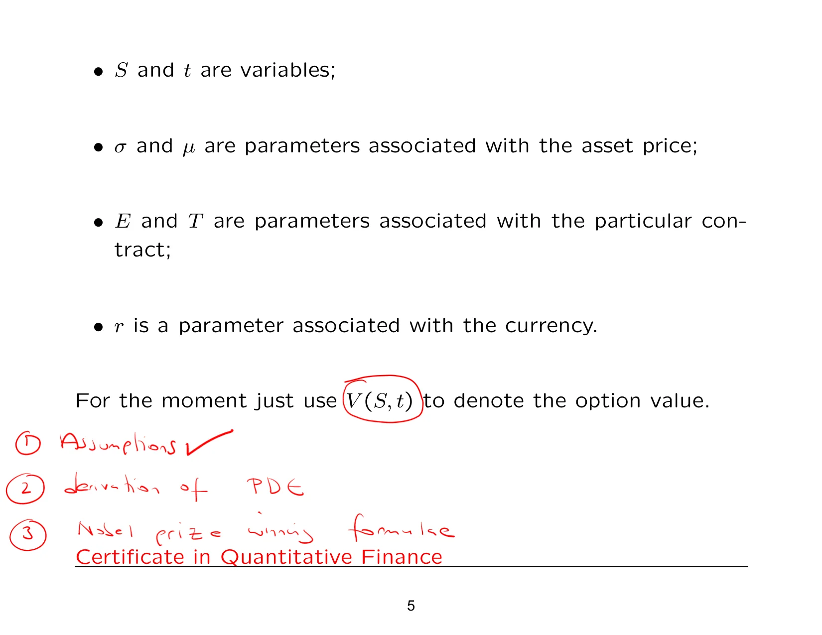
The Black-Scholes modelBlack-Scholes model The Black-Scholes model is a continuous-time framework for pricing options and other derivatives. is the one that most of you have probably been waiting for, because it seems to be synonymous with mathematical finance. What we're going to do this evening is talk about the Black-Scholes model, which comprises three things. First is the set of assumptions, second is the derivation of the PDEPDE / partial differential equation PDE stands for partial differential equation, an equation that relates an unknown function to its partial derivatives., and third is the Nobel Prize-winning formula.
There are going to be an extra set of notes to go with this. The reason is that there's a lot of working that needs to go in, or shall we say has been taken out. Otherwise, we'd have a set of slides that were three times as long. After that, we'll look at Black-Scholes formulasBlack-Scholes pricing formula / Black-Scholes formulas The Black-Scholes pricing formula is the closed-form expression for the price of a standard option under the model assumptions. for calls and puts, and we'll also look at binary optionsbinary options Binary options are options with a payoff that takes one of two possible values, typically a fixed amount or zero.. We talked about binary options when we were doing the binomial modelbinomial model The binomial model is a discrete-time asset-pricing model with two possible moves at each step. recently, also called digitals. The last thing we'll do is look at some sensitivities, courtesy of the GreeksGreeks / the Greeks Sensitivity measures for an option or derivative with respect to key inputs..
That's the plan or course of action for this evening. By the end of this evening, the whole purpose is to spend some time looking at the Black-Scholes equationBlack-Scholes equation The Black-Scholes equation is the PDE that option prices satisfy under the Black-Scholes assumptions. and pricing formulas. Everything we do this evening, and this is important, is in the framework of being able to find closed-form solutionsclosed-form solution A closed-form solution is an exact expression that can be written using standard mathematical functions and operations.. Everything that we do this evening is going to be ideal, sometimes unrealistic, but that's fine because later on we'll relax all of these one by one.
We'll look at the formulas and then understand the meaning of common GreeksGreeks / the Greeks Sensitivity measures for an option or derivative with respect to key inputs.. There is an extra thing here: expectations. We're also going to be looking at that, because that will then give us the link with Monte Carlo.
In terms of the chronology of events in mathematical finance, this had to be one of the biggest breakthroughs, generally in finance, namely the pricing of optionsoption pricing Option pricing is the task of determining the value of an option contract.. The derivation, you're going to find, is quite straightforward. We're going to use some basic ideas from finance, which you've already done, and you would have seen them in the binomial modelbinomial model The binomial model is a discrete-time asset-pricing model with two possible moves at each step., and some basic stochastic calculusstochastic calculus Stochastic calculus is the calculus of random processes, used to model and manipulate quantities that evolve with uncertainty.. That's the idea.
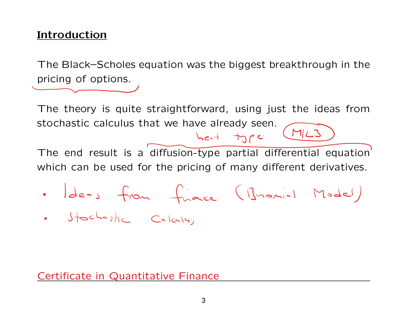
What we're going to have is a heat-type equationheat-type equation A diffusion-like partial differential equation with the same form as the heat equation., and then it's going to start looking very familiar, especially when you compare it to Module 1, Lecture 3. We've done all the hard, messy, unpleasant work, and what you're going to see is a lot of things being revisited.
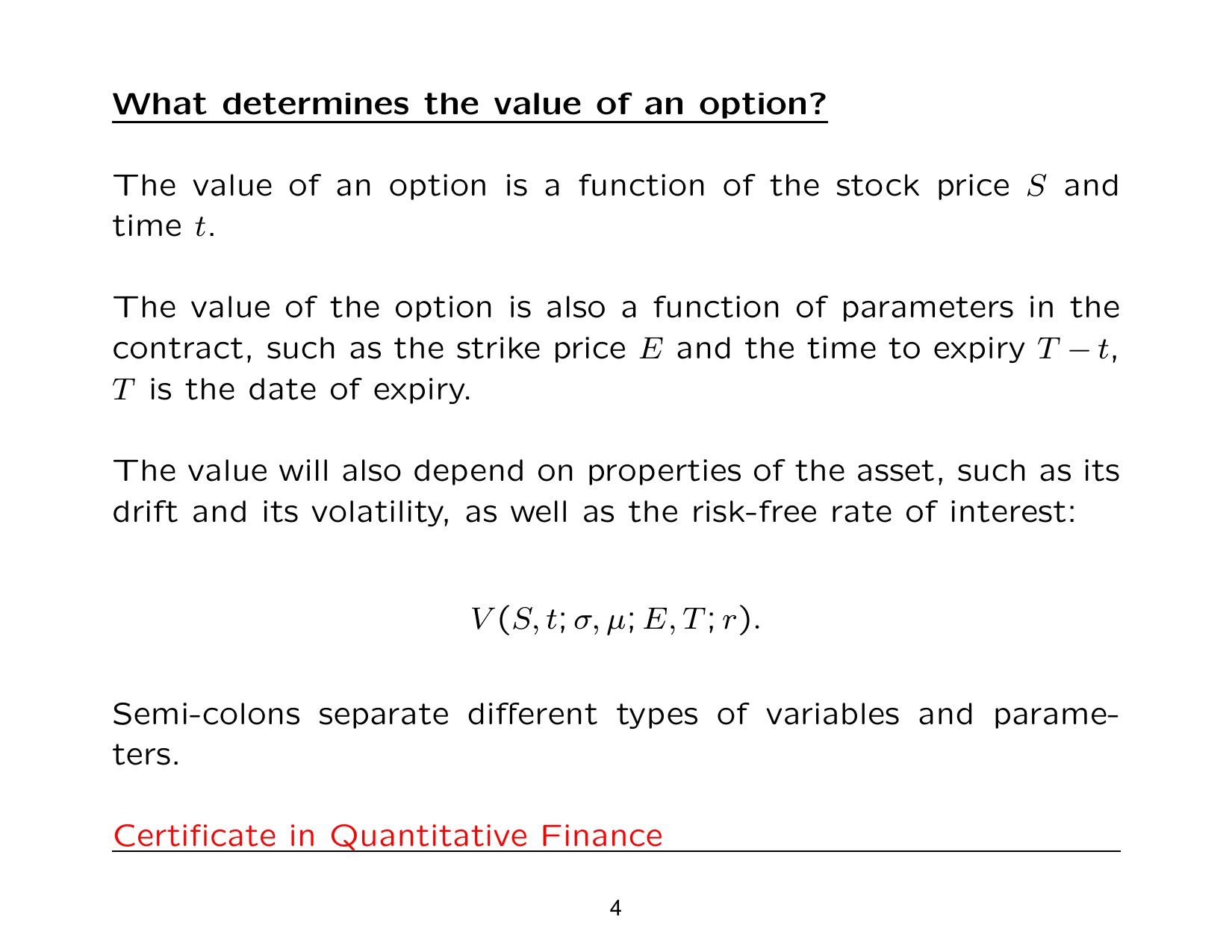
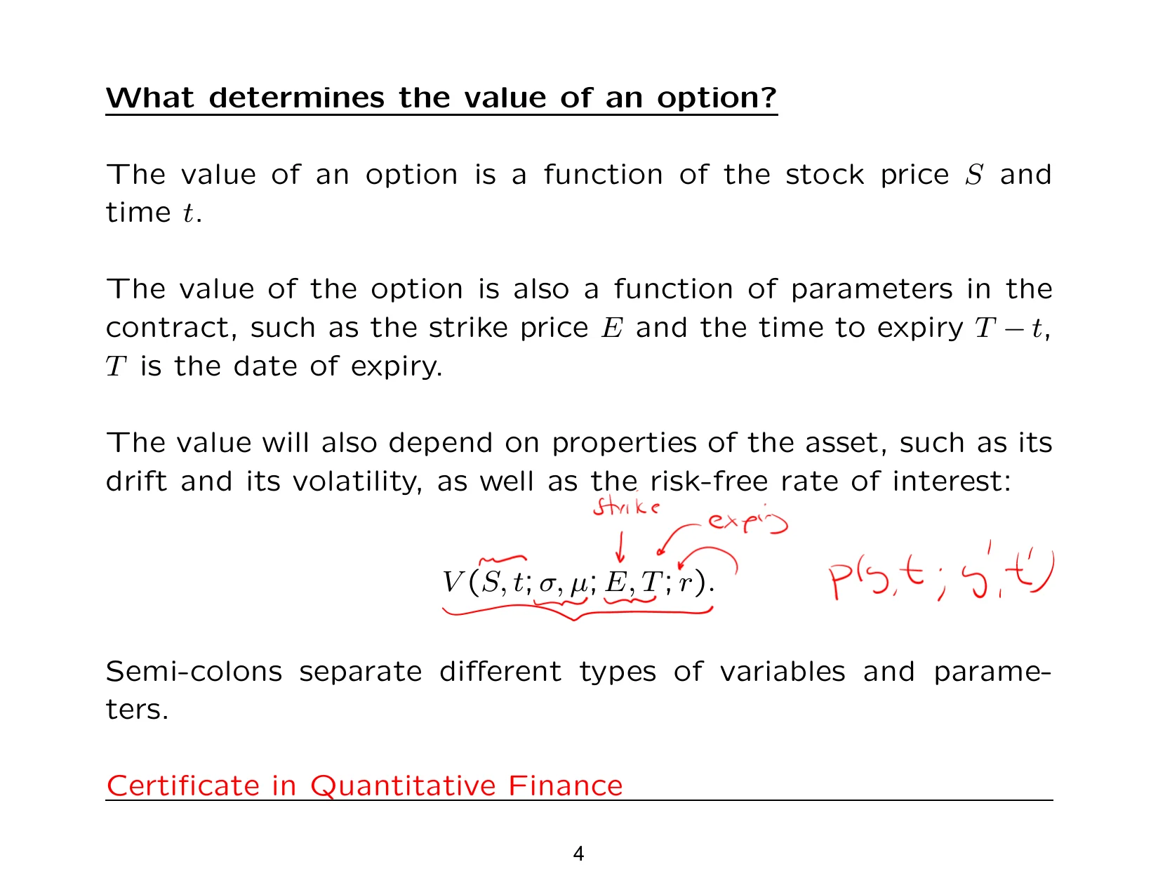
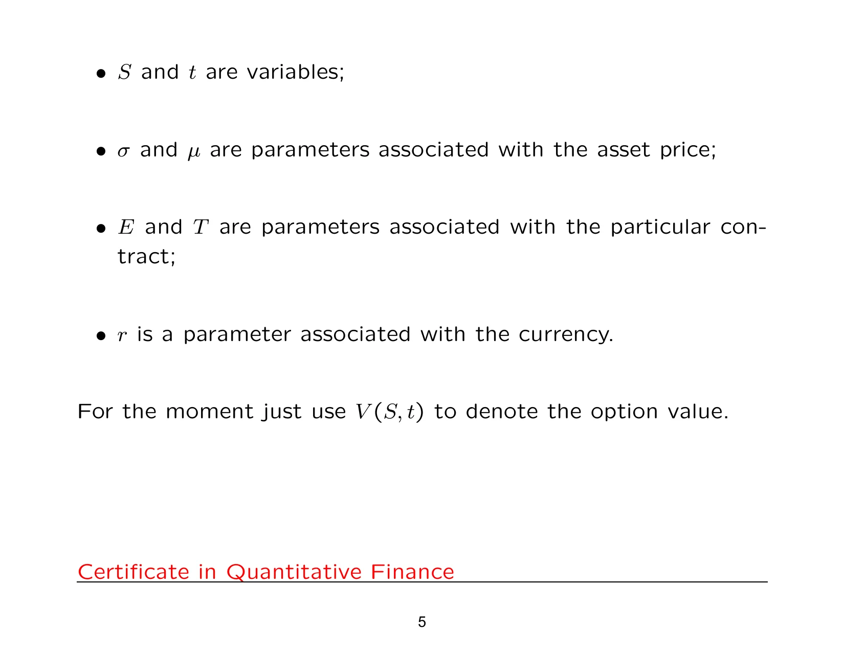
So what are the factors that determine the price of an option? Two variables: the stock and the time. Parameters associated with the underlyingunderlying The underlying is the asset or instrument on which a derivative contract is written., features of the contract, in other words strikestrike price / strike The strike price is the contract price used to exercise an option, also called the strike., expiryexpiry The time at which an option or contract matures and its payoff is settled., and the risk-free interest raterisk-free rate / risk-free interest rate The risk-free rate is the benchmark interest rate used for discounting and comparison in pricing models.. Obviously, it would look really messy if we started having to write this every time, so because only S and t are variables there, we're just going to write this down.
As far as this kind of notation is concerned, you're familiar with this. Remember when we wrote down the transition density functiontransition density A transition density is the probability density of the future value of a process given its current state.? Remember when we wrote this down? That's what we had from earlier on.
Before we go on, we're going to write down the three things that go into the Black-Scholes modelBlack-Scholes model The Black-Scholes model is a continuous-time framework for pricing options and other derivatives.. The first is the assumptions, the second is deriving the PDEPDE / partial differential equation PDE stands for partial differential equation, an equation that relates an unknown function to its partial derivatives., and the last one is the Nobel Prize-winning formula. Shall we start with the very first one then, the assumptions?
These are all very ideal. So, 1973, Black-Scholes model. You may be wondering why so old. The reason is that this is a classic, classic meaning it's robust. The same kind of ideas keep coming up over and over again, and then what we can do is relax one or two of them, or remove some of these assumptions. But we're going to start off with this, because this is what launched this famous equation.
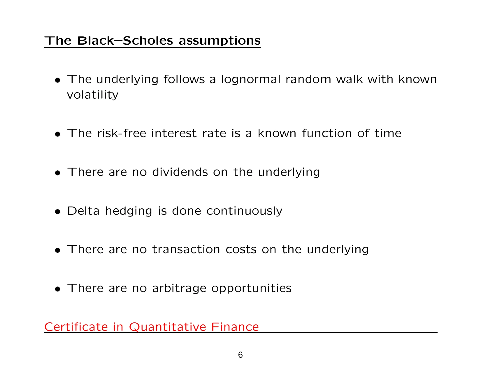
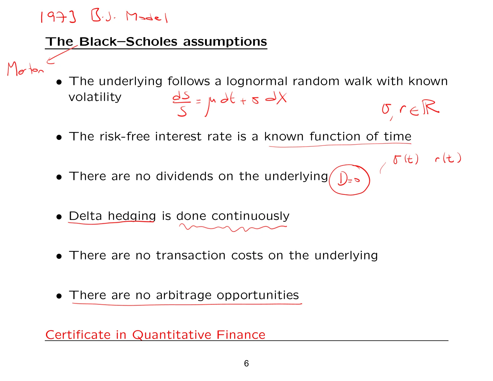
The very first one is that the stock price satisfies a geometric Brownian motiongeometric Brownian motion A random process commonly used to model asset prices, with proportional changes and continuous randomness., that is, this. That's the first assumption. The second one is that the two parameters, sigmasigma Sigma is a parameter in the model, typically representing volatility or a volatility-related quantity. and r, are constants. I know Paul's written here a known function of time; this is something that was introduced later on. At the original time of the development of the equation, it was assumed that both of these are constants. We can allow both sigma to be a function of time, as well as r to be a function of time, and for the time being we'll just assume that these are both constants.
They assumed that there are no dividends on the underlyingdividends Cash payments made by a company or asset to its holders, sometimes affecting option pricing.. There was a third person here, Merton. The people who won the Nobel Prize for Economics were Scholes and Merton, because Black had passed away. They also assumed that there were no dividends on the underlyingunderlying The underlying is the asset or instrument on which a derivative contract is written.. That was another important consideration.
Then they said delta hedgingdelta hedging Delta hedging is a strategy that uses the underlying asset to offset changes in an option’s value. is done continuously. You've seen hedginghedging The act of reducing exposure to risk by offsetting a position with another position. and you've seen the idea of short sellingshort selling Short selling is a trading strategy where an investor sells an asset they have borrowed, hoping to repurchase it later at a lower price.. Then they said frictionless marketsfrictionless markets An idealized market in which trading can occur without costs or restrictions., an infinite pool of money with which to trade. So that doesn't happen in real life. They said there are no transaction coststransaction costs Transaction costs are the expenses associated with buying or selling an asset. on the underlying, so you don't have to worry about buying and selling and paying fees. No limits to trading, no taxes. Anyone here who owns shares will know that the buying and selling of this isn't God's work; you have to pay for this. And then there's another one: there are no arbitrageno-arbitrage principle / no arbitrage The no-arbitrage principle says that prices must not allow a riskless profit from a self-financing strategy. opportunities.
Obviously, we know that short sellingshort selling Short selling is a trading strategy where an investor sells an asset they have borrowed, hoping to repurchase it later at a lower price. is allowed. You've seen examples of this, and you've also seen this in the binomial model. Over here, they said it's done continuously. Obviously, anyone who does this for a living will know that you can't do this continuously. But these are all ideal and, dare I say, unrealistic assumptions, simply so that they could come up with an equation that they could solve by hand.
Remember, 1973 is when this paper was published. So if you go back a couple of years before that, you can probably guess what the availability of computational power would have looked like: probably very scarce. So that's the reason why I keep reminding you, before anyone thinks, hang on a second, how can you have this because it doesn't exist in real life? We're not worried about real life to that extent this evening. There are some other assumptions as well, but these are the big ones. This is assumption number one, the underlying assumption number one.
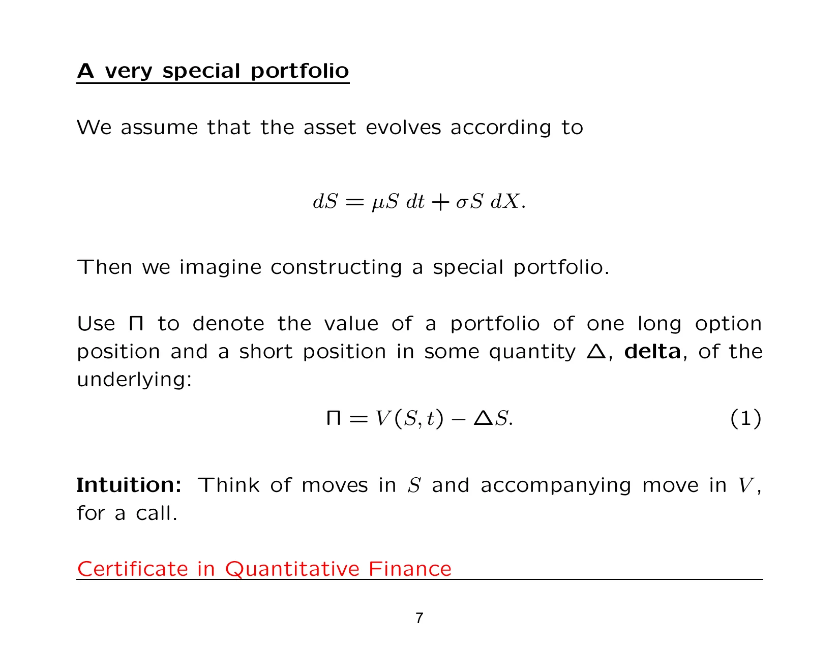
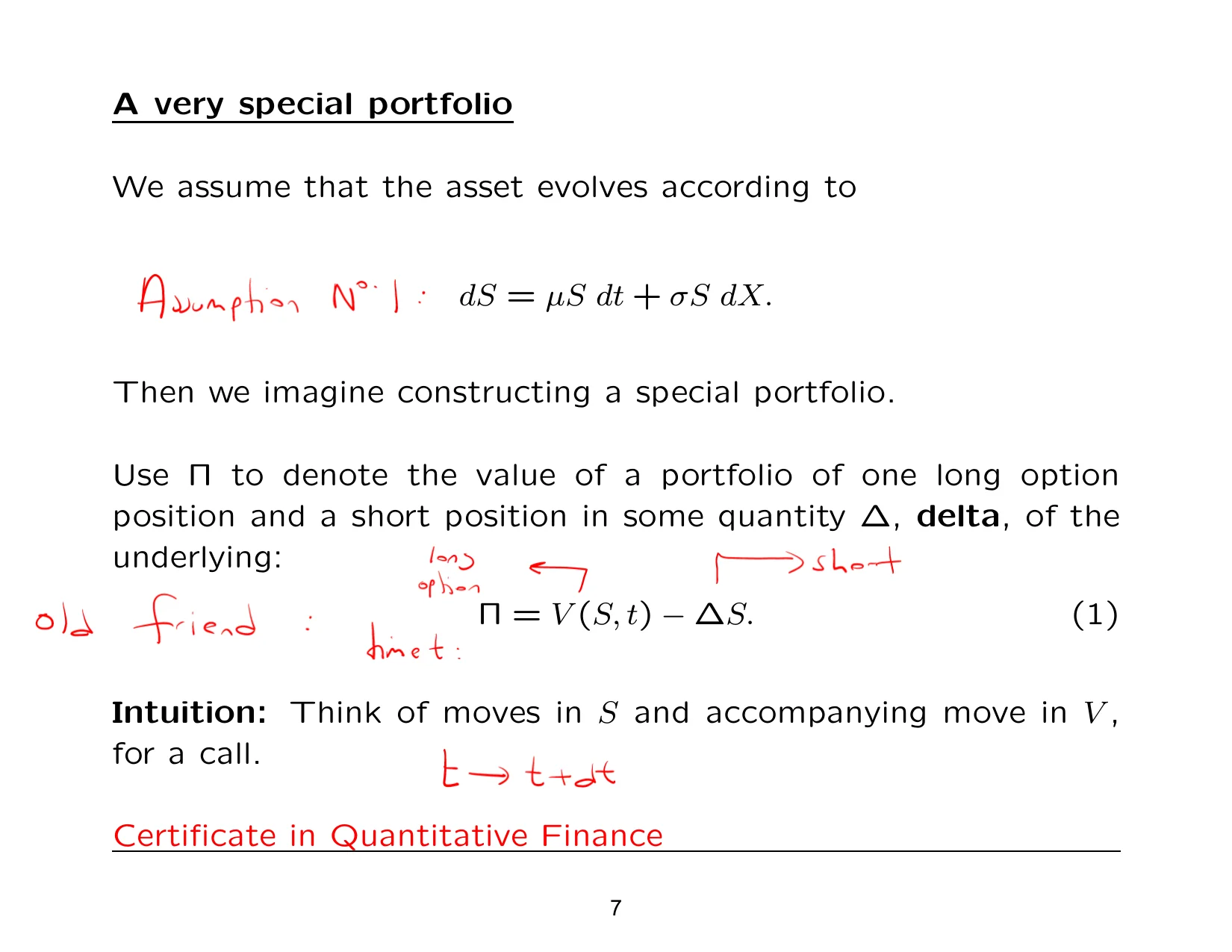
Then we look at an old friend. Would you agree that you've seen equation one before? Long an option, short an amount of stock. You see, when you get to this lecture, because you've done all the hard, fiddly work before, this becomes really straightforward, because you've seen all the intuition and the justification for this from when Paul did the binomial model, that is, the second lecture. So at this point, everything comes together in a nice, systematic way. These are all familiar things to you. This is at time t.
If this is at time t, then the obvious question you may ask is what happens to the portfolio across one time step. In other words, how does it change? We change it keeping deltadelta Delta is the sensitivity of an option’s value to a small change in the underlying asset price. fixed during the time step, and that's the reason why we end up with this, because what we're doing is dV minus delta dS. Delta is fixed, so we end up with this.
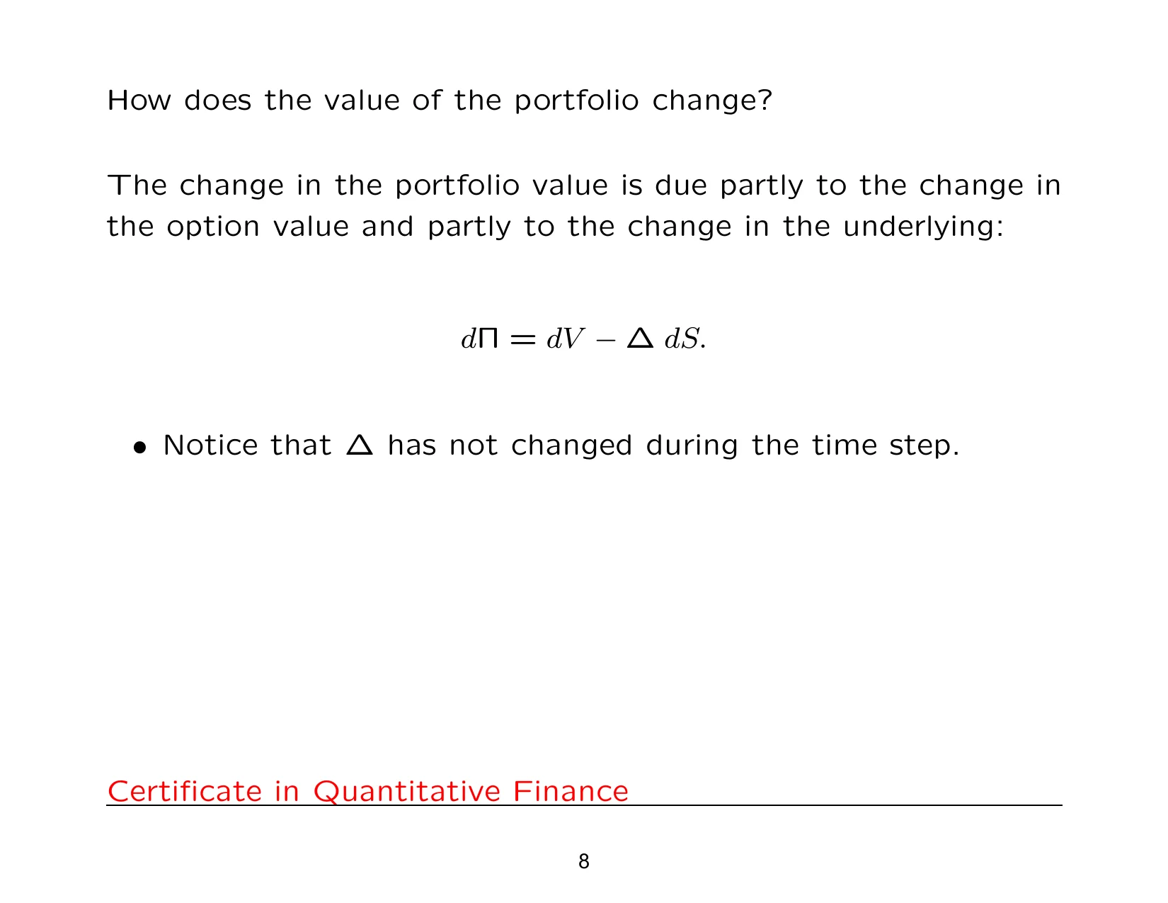
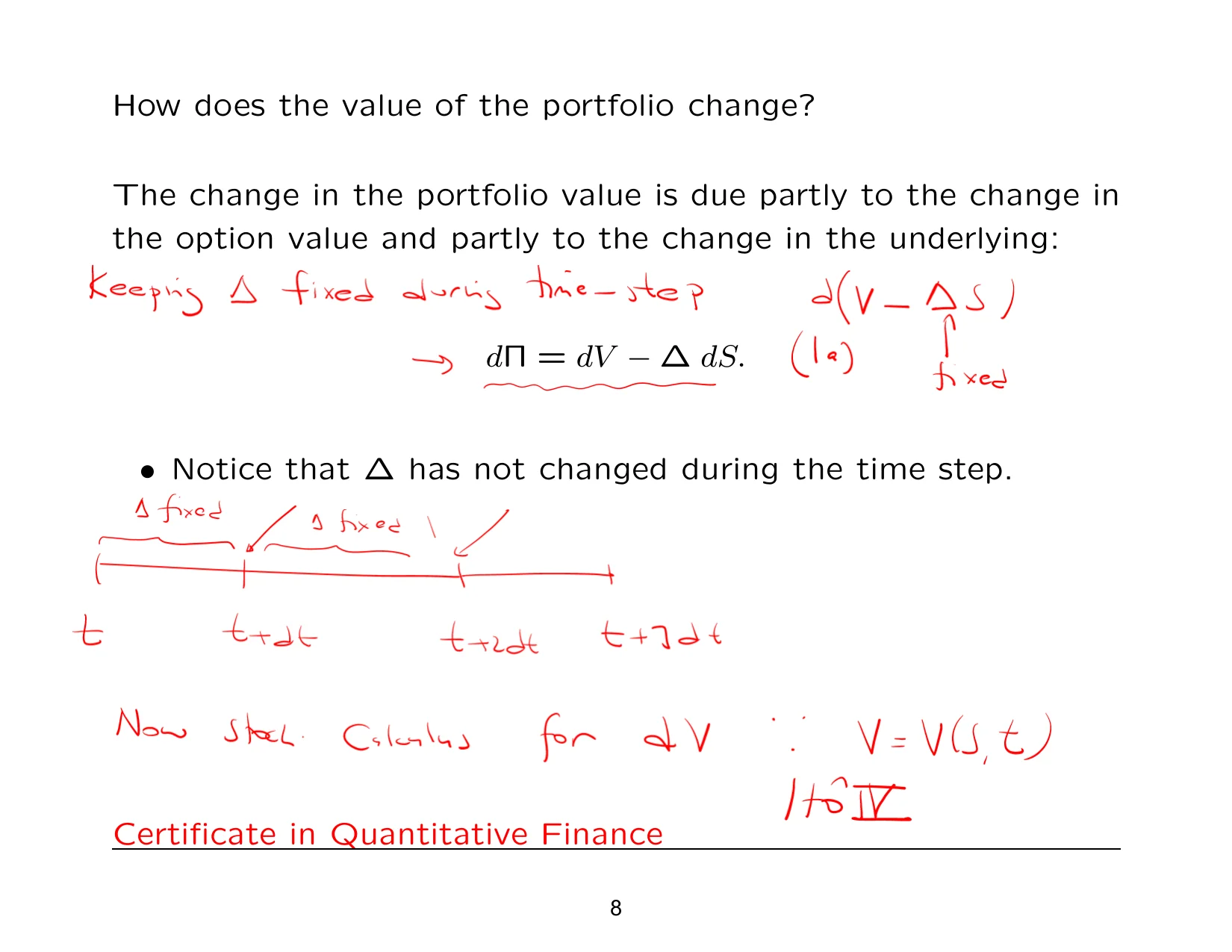
And what does it mean for deltadelta Delta is the sensitivity of an option’s value to a small change in the underlying asset price. to be actually fixed? It says here, note that delta has not changed during the time step. It's fine, because when we come back to the start of the next time step, then we'll change it. So when we talk about delta being fixed, we only mean that it's fixed across this, that's all. Across here it's fixed, but not here. We recalculate it, fix it again, we recalculate it, and so on. That's what that means, and that's the reason why we get delta dS.
So those were the finance ideas for the time being.
That's all. So across here, it's fixed, but not here. We recalculate it, fix it again, recalculate it, and so on. That's what that means, and that's the reason why we get delta dS. So those were the finance ideas for the time being.
Now, stochastic calculusstochastic calculus Stochastic calculus is the calculus of random processes, used to model and manipulate quantities that evolve with uncertainty.. Stochastic calculus for dV, because V is a function of S and t. So which version of Itô do you think we're going to use now? We're going to use version 4. So Itô 4Itô expansion / Itô 4 Itô expansion is the stochastic-calculus analogue of Taylor series for functions of processes driven by randomness., that's the version we're going to use.
But the interesting thing you're going to see is that Paul doesn't actually write out the whole version, and there is a reason for that. The reason is that some of the terms are going to cancel out, so he just doesn't bother. You'll see what I'm talking about in a second.
Again, all familiar stuff. The only difference is that Paul hasn't replaced this. Normally we would replace this, wouldn't we? If I squeeze it in here, what does that become? Oops, I've forgotten a term there. We've written it out in full; this is what it becomes.
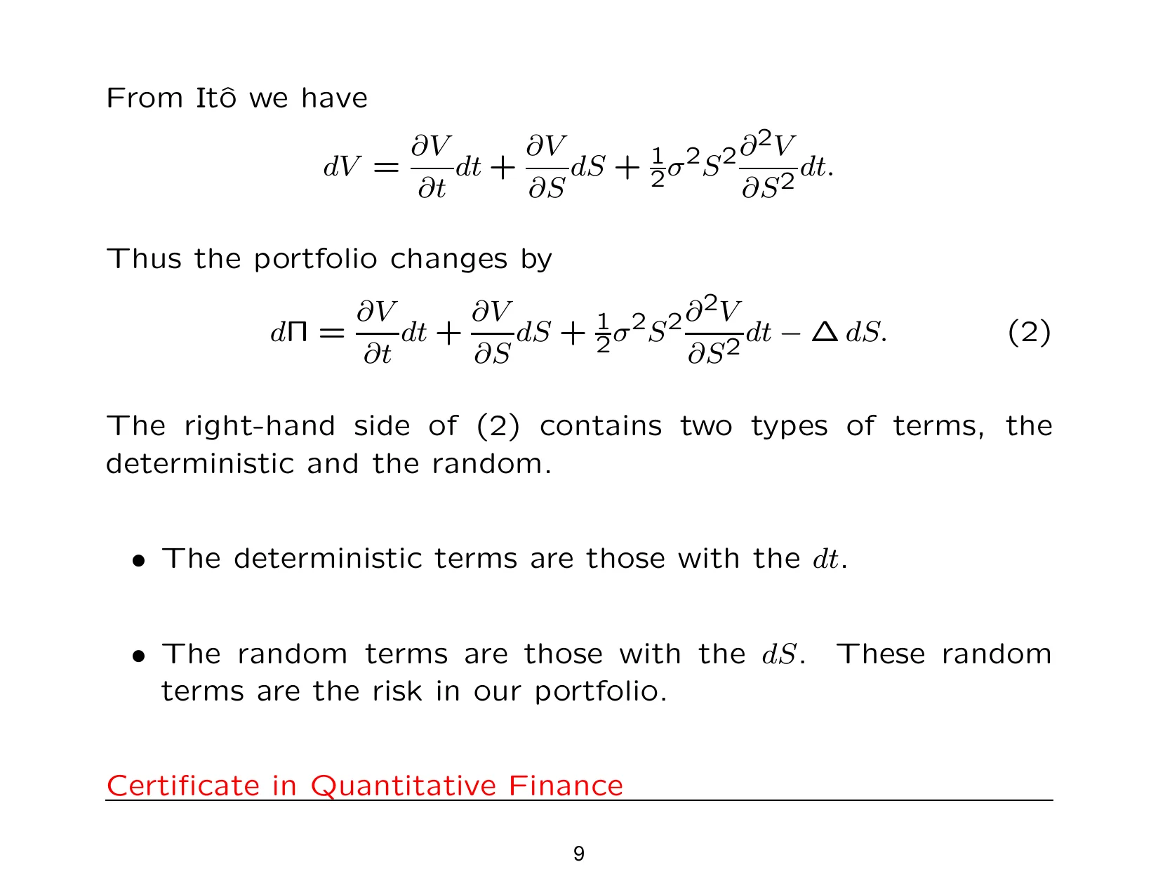
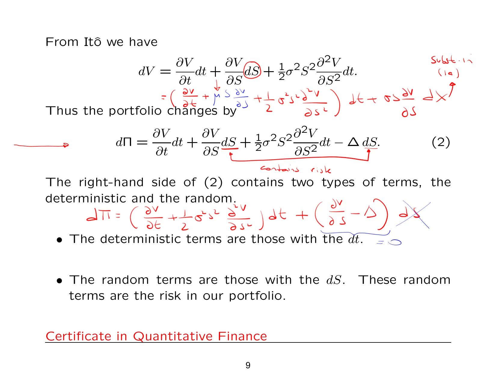
So if we now substitute all of this into, is it equation 1? No. Shall I call this 1a? Let's call that equation 1a. Substitute in, so we substitute this into equation 1a, and this is what it becomes. Again, the only difference is that Paul hasn't replaced that. Otherwise, everything else is the same.
That's the portfolio change. So we now have a combination of things with risk and things that are deterministic. We know that the risk is captured in here; it contains risk. Now that we have identified it, the next question is: is there any way of getting rid of risk?
We can, because if we write this down as follows, dV by dt plus a half sigma squaredsigma Sigma is a parameter in the model, typically representing volatility or a volatility-related quantity. S squared d squared V by dS squared, those are all the coefficients of dt, plus dV by dS minus delta, all multiplying dS. Then we argue that if we could somehow get rid of the risk by setting this equal to zero, this term vanishes. So that gives us a choice for delta.
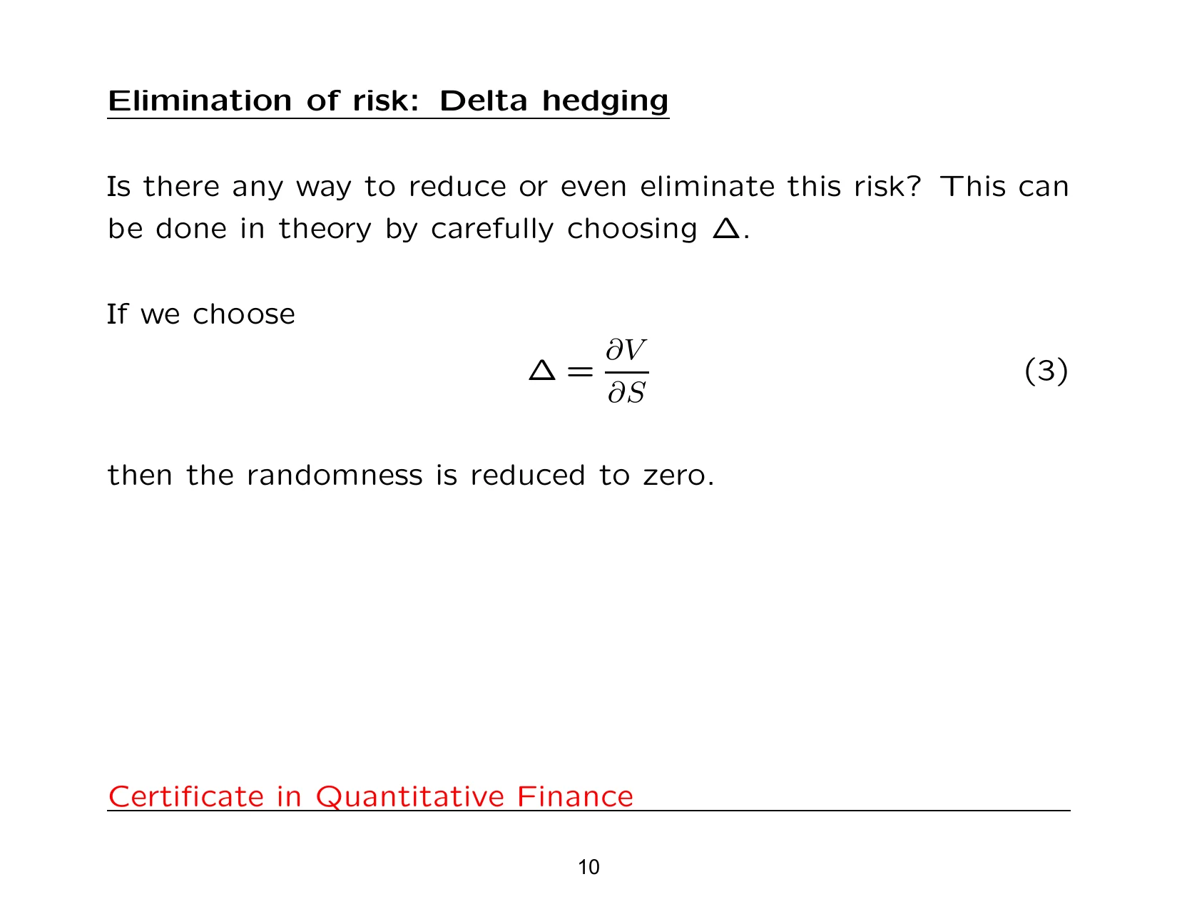
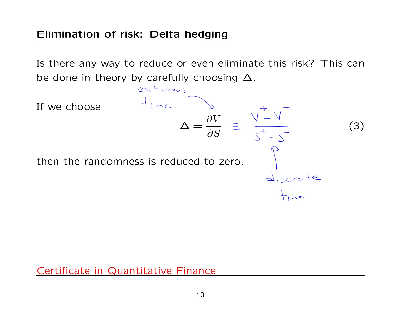
So your next step would be to say: to eliminate risk, set delta equal to dV by dS. Now look what happens when I write down next to it what we had in the binomial model. Remember, that was discrete time; this is continuous time. See that? It all makes sense. So there's our choice: delta is equal to dV by dS.
Remember, when we talk about reducing risk, we say it's hedginghedging The act of reducing exposure to risk by offsetting a position with another position.. The perfect elimination of risk by exploiting correlation between financial instruments is an example of delta hedgingdelta hedging Delta hedging is a strategy that uses the underlying asset to offset changes in an option’s value.. And the fact that, at the end of each time step, we're going to be recalculating the delta means that this whole thing is an example of a dynamic hedging strategydynamic hedging strategy A hedging method in which positions are updated repeatedly over time to maintain the desired risk exposure..
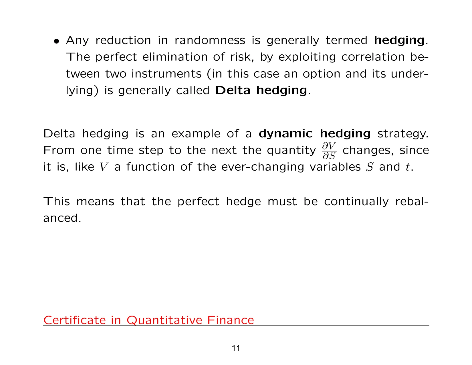
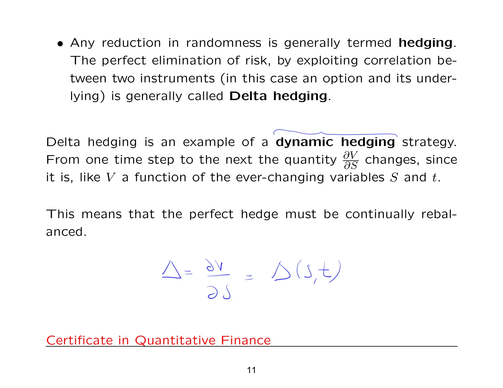
The fact that the delta is constantly being re-evaluated, rebalanced, recalculated. Because if delta is dV by dS, that tells us that delta is in fact a function of both S and t.
Once you've got delta equal to dV by dS, something interesting happens. Equation four is what's left. The obvious thing is that the risk has gone. First of all, we notice that there's nothing capturing the dX term. But more importantly, we notice something else: if dS is gone, randomness is eliminated, and as a consequence of that, mu is also gone. In other words, the real-world driftreal-world drift Real-world drift is the expected rate of change of an asset price under the actual probability model. mu of the stock price returns is gone.
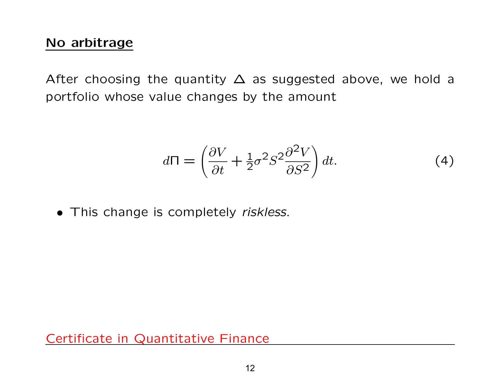
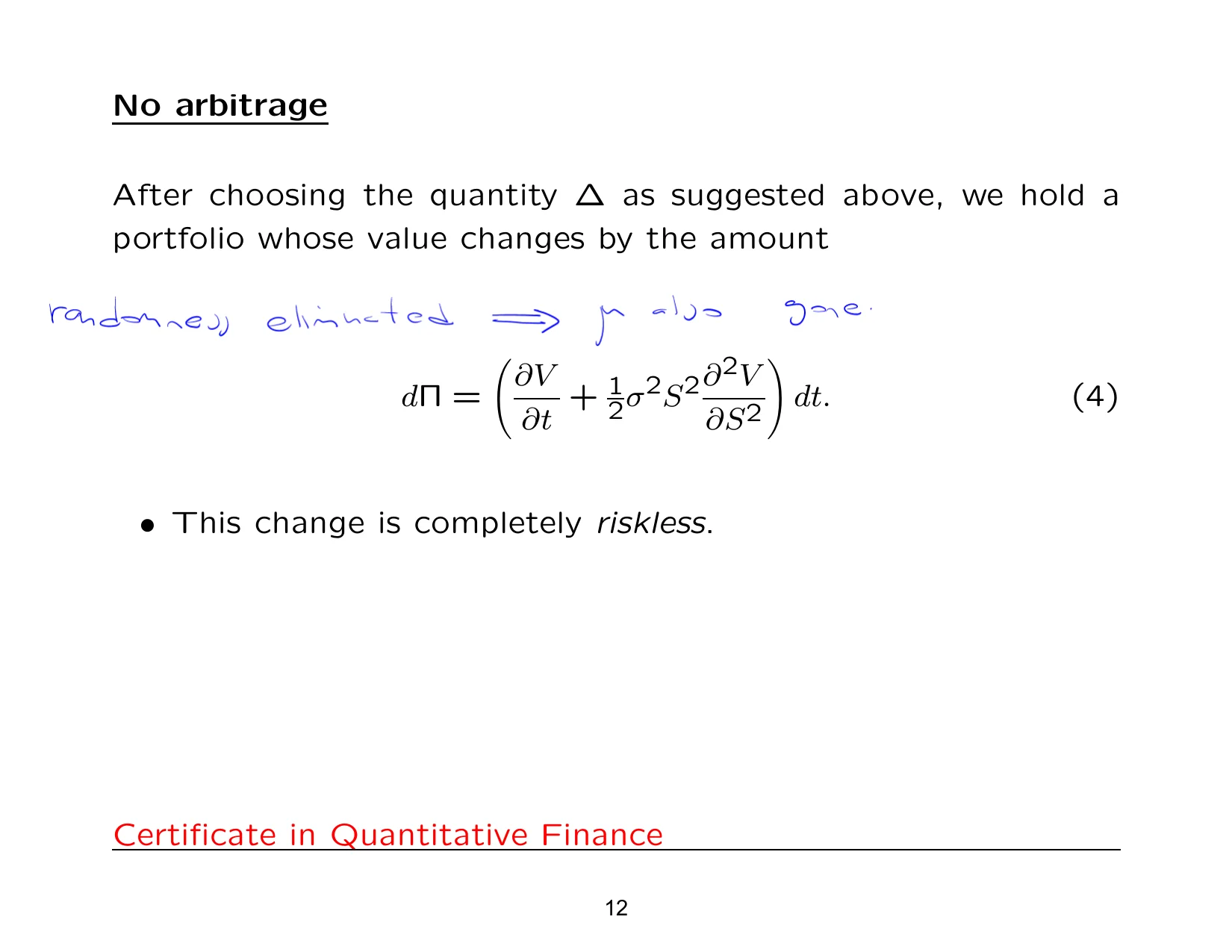
So two interesting things have happened. I would say that dX disappearing is less interesting than the fact that mu is also gone. So now, because risk has gone, remember we kept talking about this in the binomial model, we can now appeal to the no-arbitrage principleno-arbitrage principle / no arbitrage The no-arbitrage principle says that prices must not allow a riskless profit from a self-financing strategy..
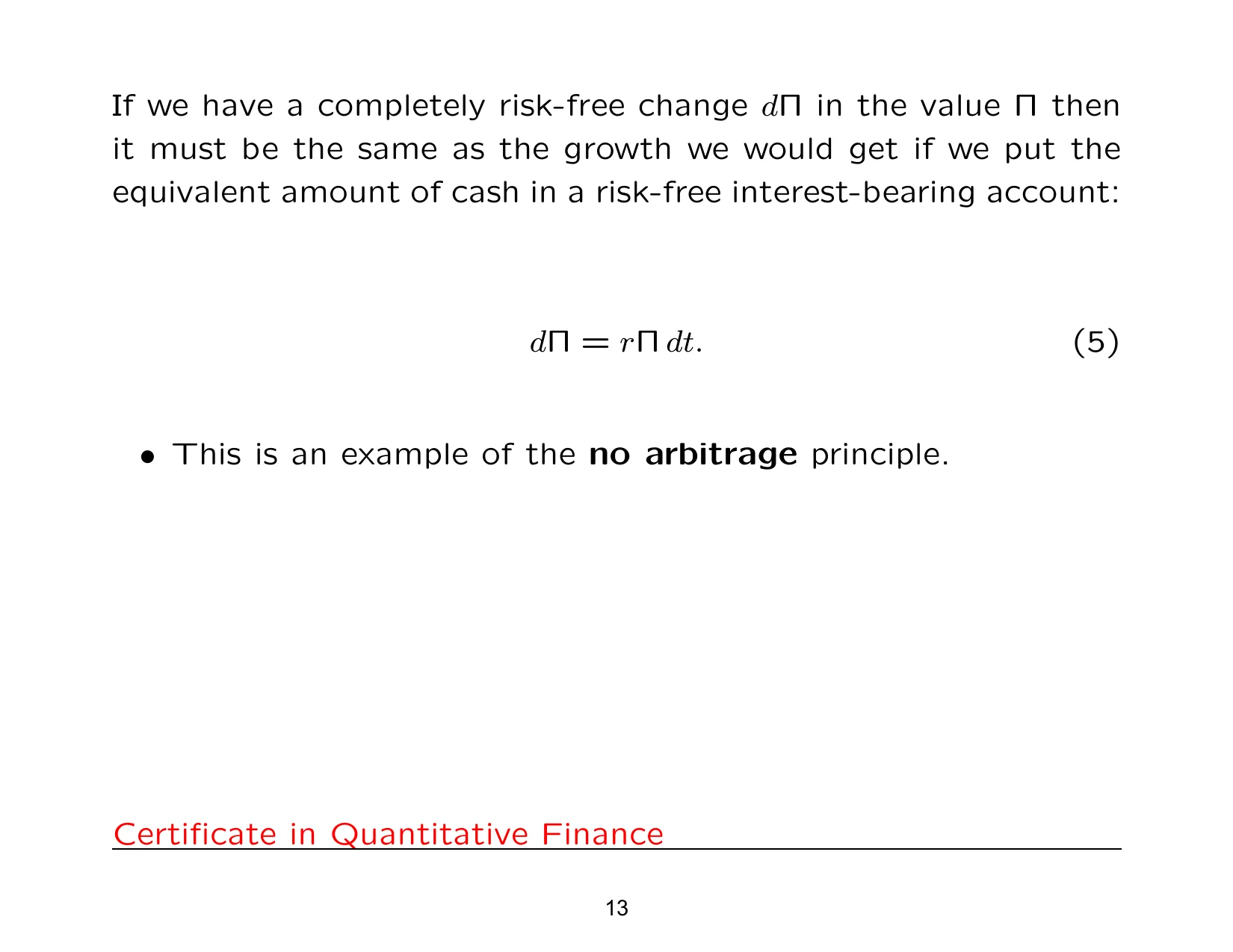
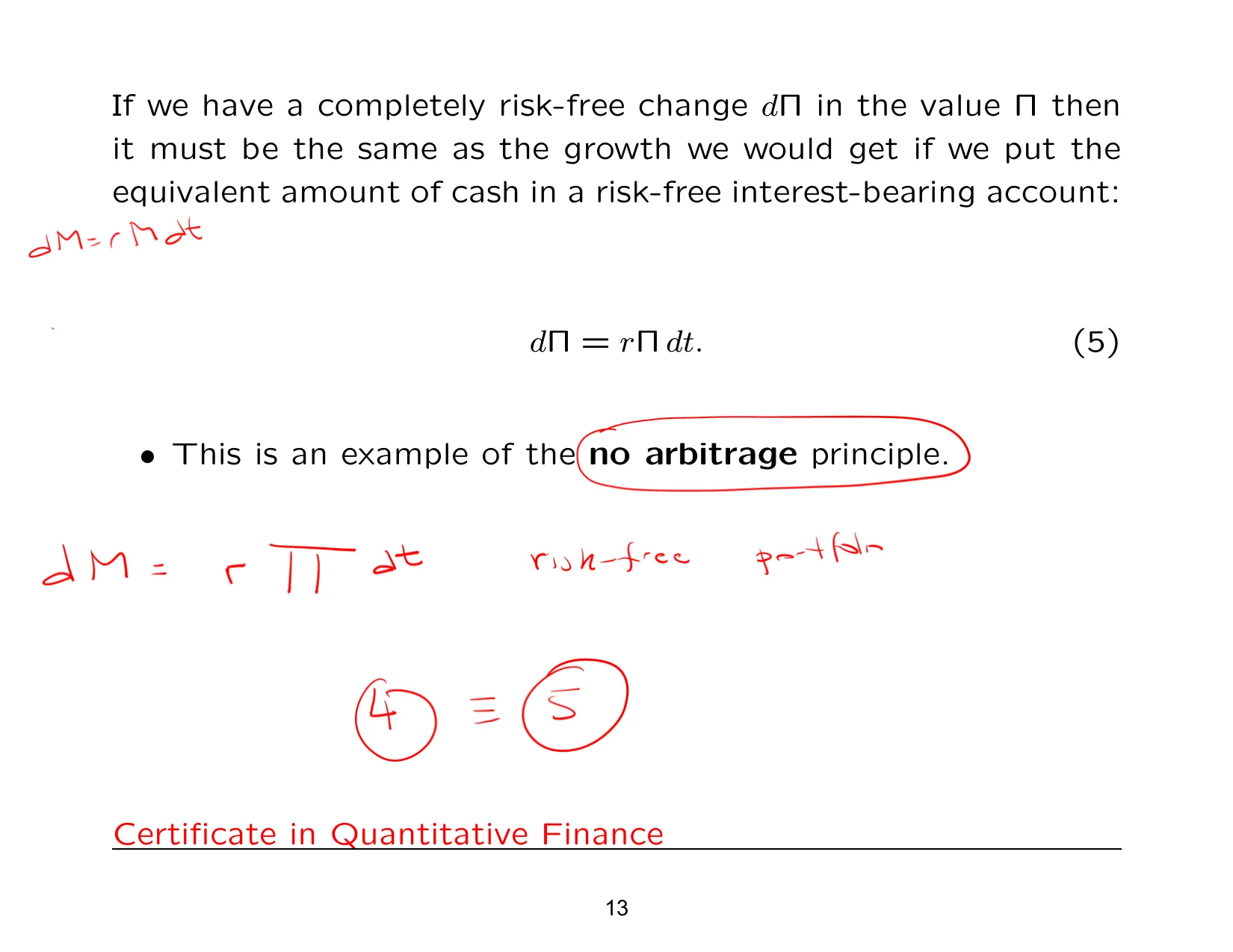
We've got equation four. Equation four is what our portfolio change looks like. So the question is: is there another risk-free portfoliorisk-free portfolio A risk-free portfolio is a portfolio whose value is designed to be free of uncertainty over a short time interval. out there? And there is: money in the bank. We know that pi is worth some financial amount. Let's suppose we take that and open up a risk-free interest-rate-bearing account, which is receiving interest at the rate r across each time step dt.
You've seen this equation before. For example, dM is rM dt, and that's what gives us compounding. So that tells us that across a time step, this is what it's equal to: dM is equal to r pi dt. So this is also a risk-free portfoliorisk-free portfolio A risk-free portfolio is a portfolio whose value is designed to be free of uncertainty over a short time interval., money in the bank.
Because we're appealing to the no-arbitragearbitrage Arbitrage is a pricing inconsistency that allows a profit without net risk in an idealized market. principle, it means that these two quantities have to be the same. So four is equivalent to five. If it wasn't, then we'd have arbitrage. People wouldn't put money in the bank; they'd create a delta-hedged portfoliodelta-hedged portfolio A portfolio constructed to offset price sensitivity to the underlying asset, at least for small moves., long an option, short an amount of stock, and make more money than the risk-free raterisk-free rate / risk-free interest rate The risk-free rate is the benchmark interest rate used for discounting and comparison in pricing models..
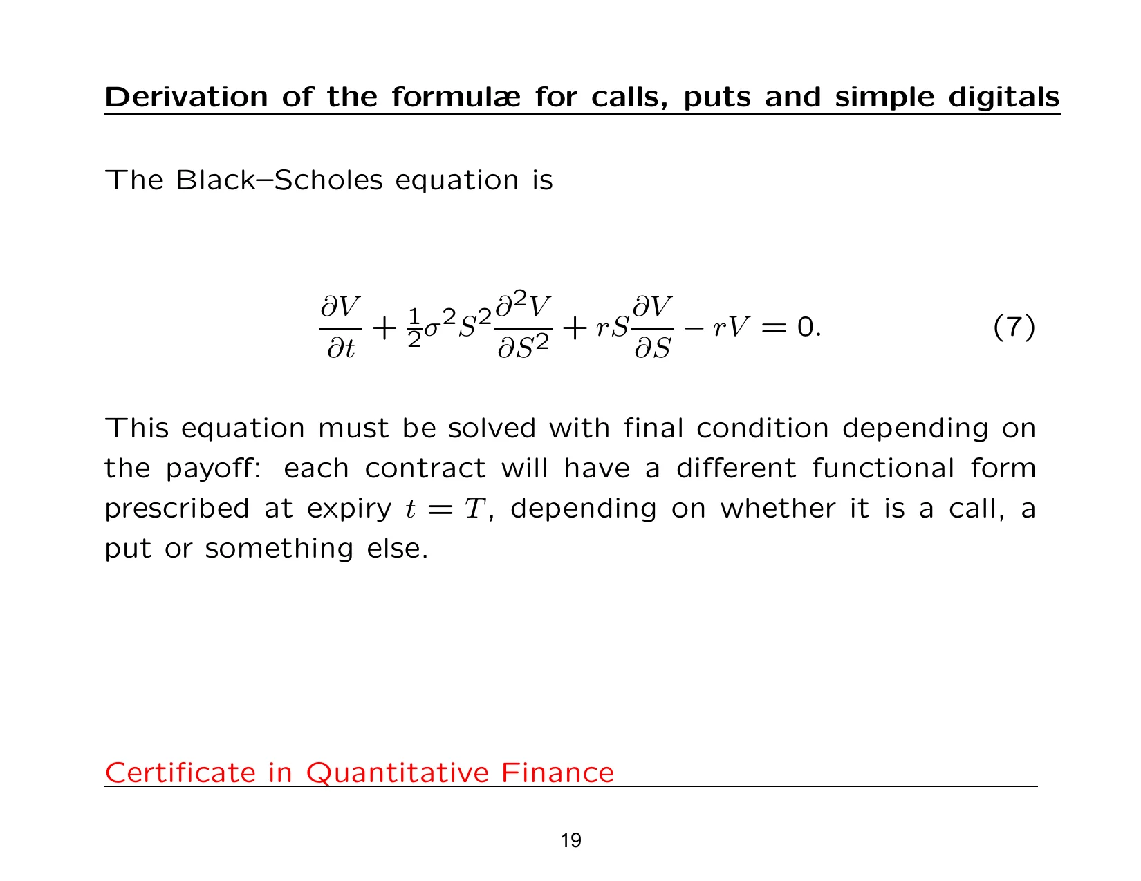
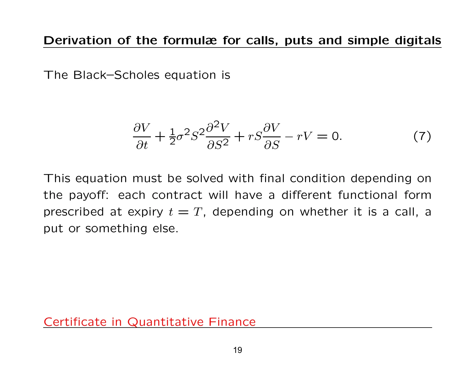
There we go. This was equation four, wasn't it? And this was five. Remember, that's pi. So d pi is equal to this, and it's also equal to that. And after we rearrange, this is the famous Black-Scholes equationBlack-Scholes equation The Black-Scholes equation is the PDE that option prices satisfy under the Black-Scholes assumptions.. Equation six is the Nobel Prize-winning Black-Scholes equation.
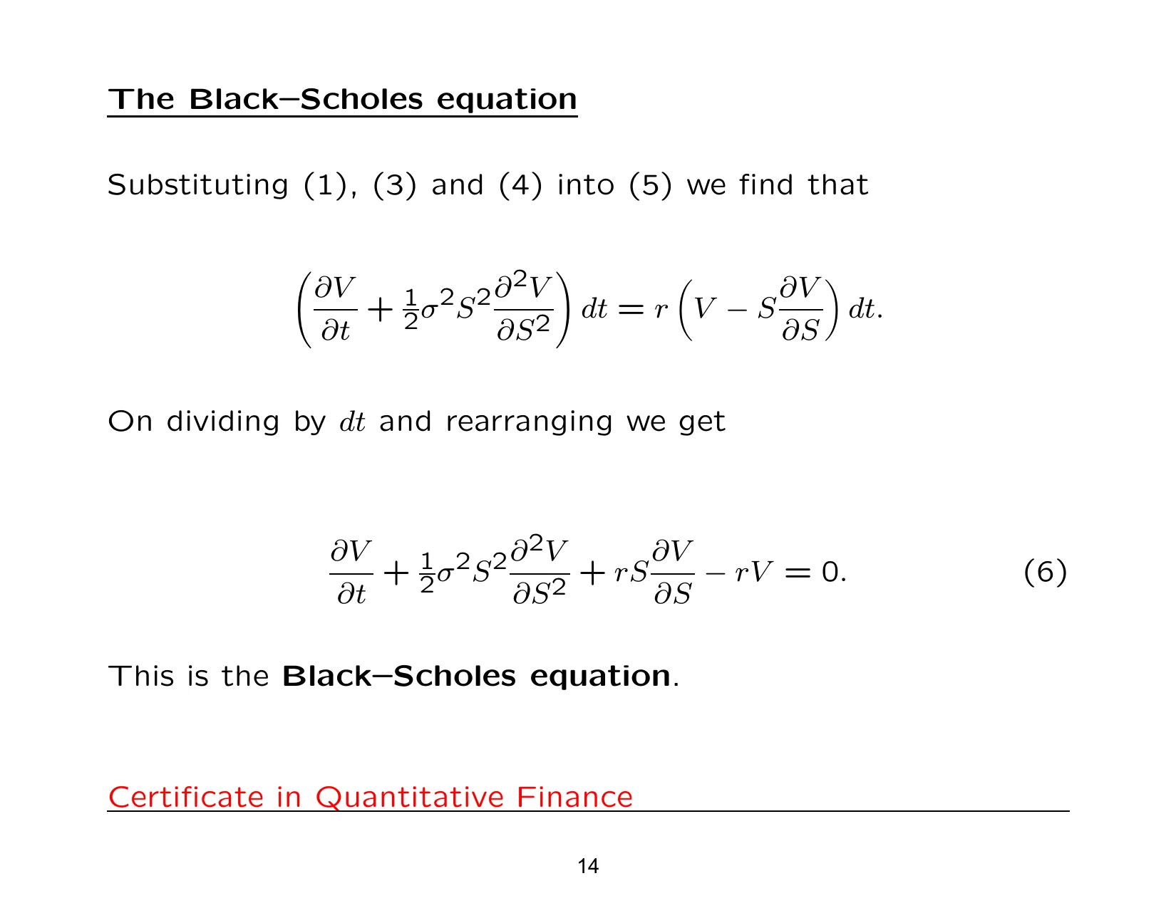
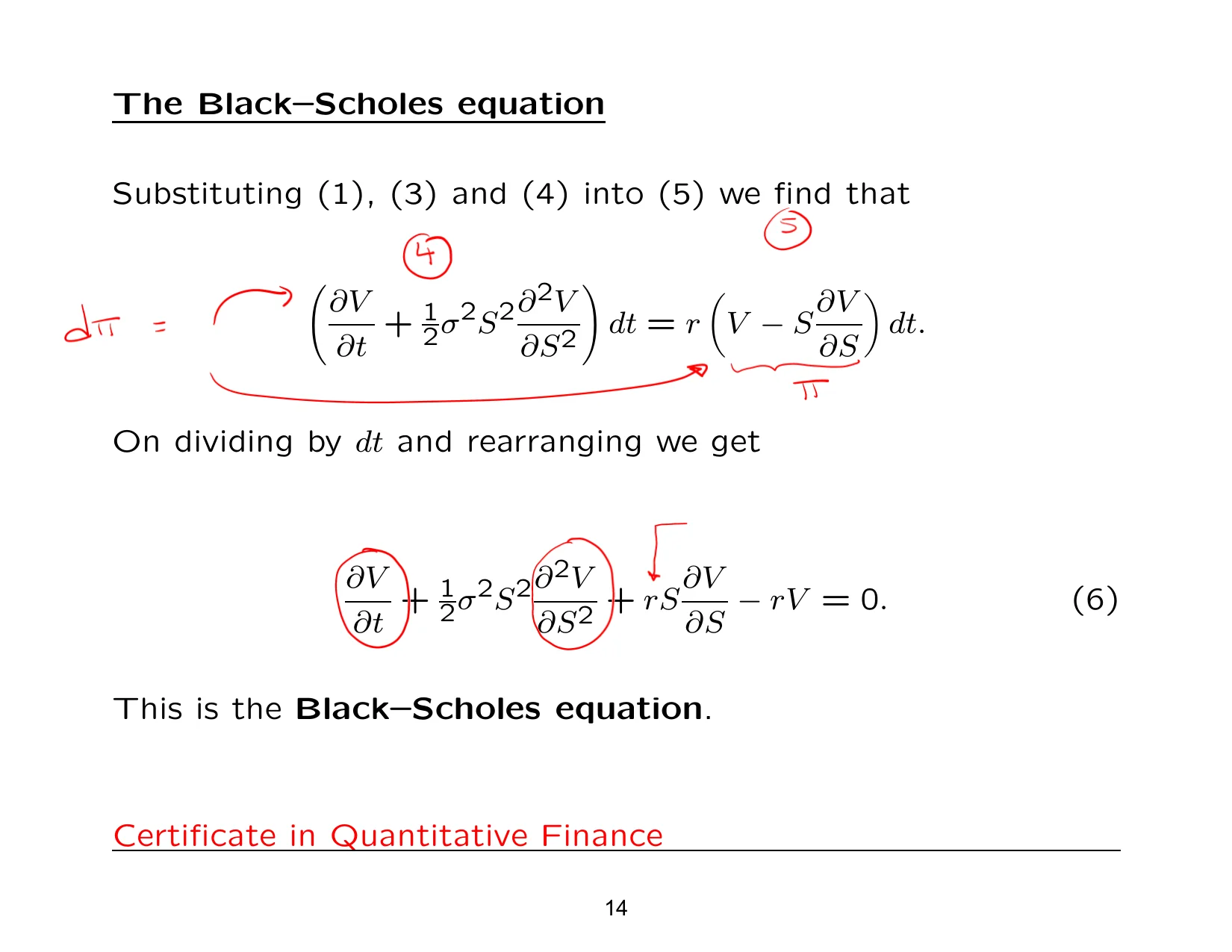
Now, there are many, many ways of arriving at this equation. This is just one of many. Would you agree that that derivation was very straightforward? We used stochastic calculus and some ideas from finance. Any questions on that?
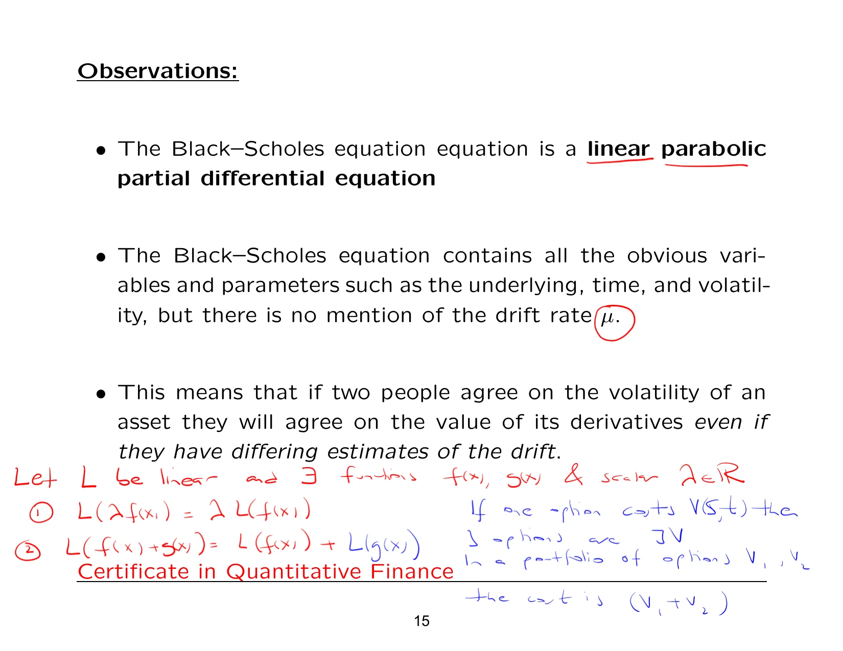
And the reason why it's a heat-type, or diffusion-type, equation is that it is first order in time and second order in the underlying variable. That's what makes it diffusion, or heat. What about properties of this equation? We know it's linear, because if you look at the coefficients of each of those terms, none of them entail a V or any of its derivatives. It's parabolicparabolic Parabolic describes a class of partial differential equations with one time derivative and second-order derivatives in space. because it's first order in time and second order in the underlying stock price.
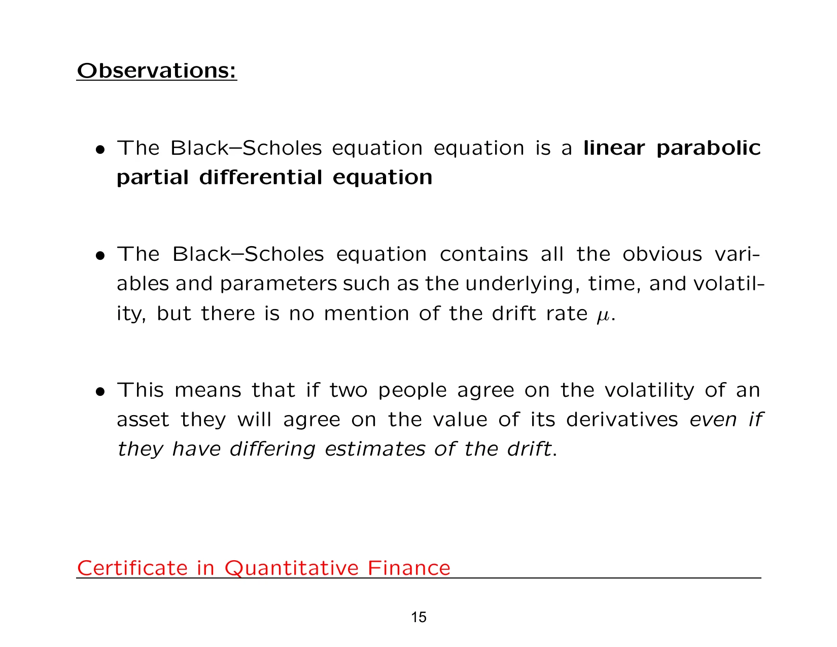
Could you explain what it means for mu to be gone? Well, there's no mu here. The dS has vanished. The dS had a mu term in there, and now it's gone as a result of us delta-hedging. And what's replaced it is the risk-free interest rate instead, r.
So our stocks are not growing according to their respective drifts, but the risk-free interest rate, which is r. And that's from the insistence on no arbitragearbitrage Arbitrage is a pricing inconsistency that allows a profit without net risk in an idealized market.. Exactly what you saw in the binomial model. Same kind of thing, but what you're now seeing is everything in continuous time. You've seen this already in discrete time.
Now, if you want to see more of the working, the version you get from me will have these steps. But if we go back here, remember I wrote the mu here? Remember I've got this full version there? If you substitute this version into d pi, you will see the mus actually cancelling out in real time.
It says here that the Black-Scholes equation contains all the ingredients you'd expect to see, but there's no mu. The mus vanish as a result of the hedging. And what this means is that if you and I agree on the volatilityvolatility Volatility is a measure of the size of price fluctuations in an asset or model., but we differ on the drift ratedrift rate The expected rate of change of a stochastic process over time., then we have to agree on the option priceoption price The option price is the value at which an option is assumed or observed to trade.. We have to get exactly the same.
Because, and this is one of the nice things about derivative pricingderivative pricing The process of valuing a derivative contract using a mathematical or financial model., you don't have to worry about one parameter. Now, with Sebastian, remember you did portfolio optimisation, so you had two parameters. You had sigma and you had mu. And obviously it's nice that we have one less parameter to worry about. But the fact that the most difficult parameter to calculate in finance is sigma doesn't actually make it that much less difficult for us.
Now, what I'm going to do is, I'm going to do something, I'm going—
And obviously it's nice that we have one less parameter to worry about. But the fact that the most difficult parameter to calculate in finance is sigma doesn't actually make it that much less difficult for us. I'm going to give you an insight into what the idea of linear means when we talk about linear.
Let L be linear. Then there exist functions f(x), g(x), and a scalar lambda. First of all, it means that if I have L of lambda f(x), this is equal to lambda times L of f(x). That's scalar multiplicationscalar multiplication Scalar multiplication means multiplying an object by a scalar, or ordinary number.. The second property is that L acting on the sum is the same as the sum of the individual operations: L of f(x) plus g(x) equals L of f(x) plus L of g(x).
How can we now equate this to what we mean in option pricingoption pricing Option pricing is the task of determining the value of an option contract.? So if one option costs v(x), then three options are three times v(x). That's the first property of linearity. The second property is saying that in a portfolio of options, say v1 and v2, the cost is v1 plus v2. That's what it means for us to be linear. That's a quick short note on linearity.
If I recall correctly, Sebastian is claiming that mu is more challenging to get than volatilityvolatility Volatility is a measure of the size of price fluctuations in an asset or model.. Yes, I was thinking that. Does it mean zero correlation? No, the idea of linearity doesn't have any bearing on whether something is correlated or uncorrelated. Linearity is a separate mathematical property.
Before we actually look at solving this equation, let's just have a slight embellishment here. We've already seen that one of the assumptions in the Black-Scholes equation was the idea that the underlying had no dividendsdividends Cash payments made by a company or asset to its holders, sometimes affecting option pricing.. In real life, dividends are paid discretely at certain points throughout the year. What mathematicians wanted to do was get a feel for what the impact of a dividend payment is on the price of an option.
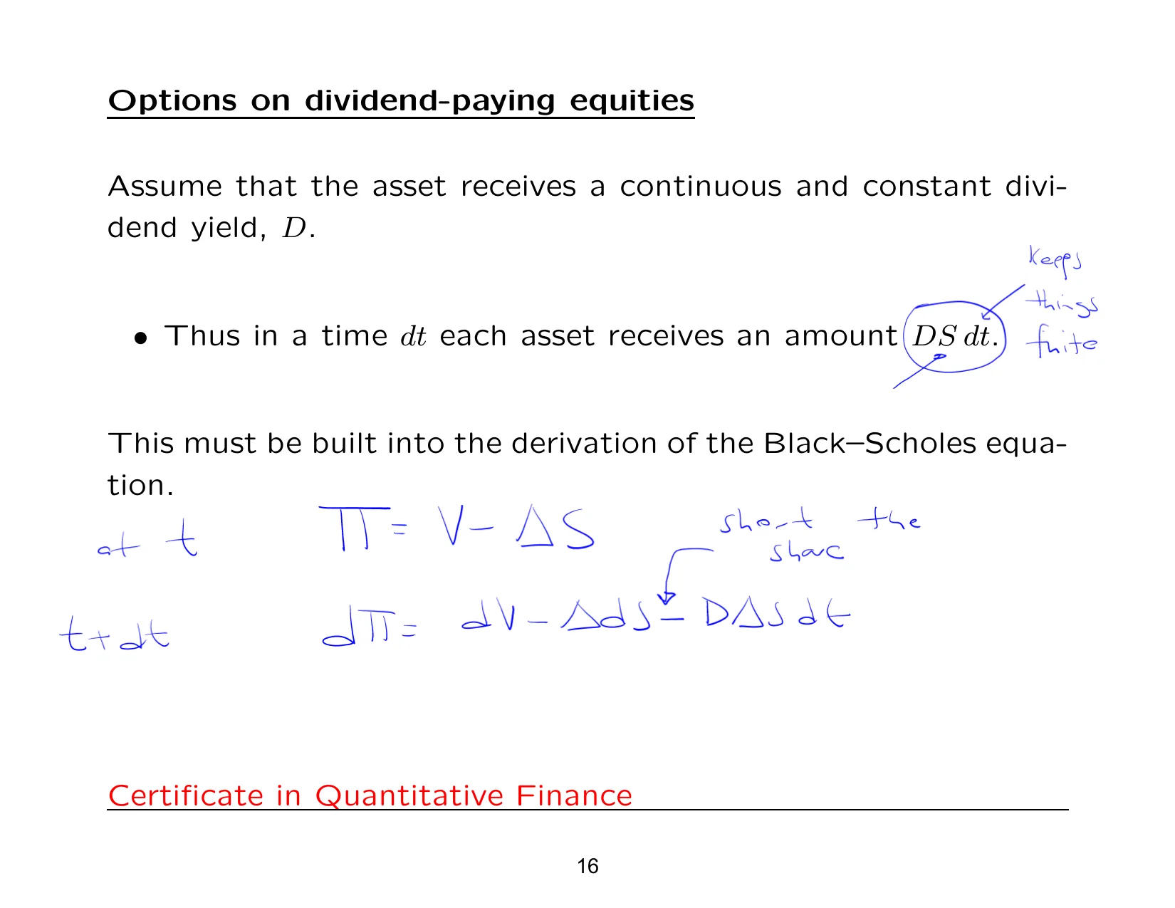
They came up with another ideal assumption. The ideal assumption was that the asset receives a continuous and constant dividend yield Dcontinuous dividend yield / continuous and constant dividend yield D Continuous dividend yield is a dividend rate paid continuously rather than in discrete amounts.. In other words, throughout the life of the option, you've got this D which has been chopped up into small bits and is being paid out across each time step. Obviously, it doesn't exist like that in real life.
Which means that across each time step, the asset receives this amount. And what the dt does here is it keeps things finite. That's what's being paid across. So we start off with exactly the same setup. That's at time t. Then we go to t plus dt, and the change is going to be dV minus delta dS. But because we're getting this amount, there's also going to be a d delta S dt term, so minus d delta S dt. Why the minus? Because we're short the share. That's going to leave our portfolio.
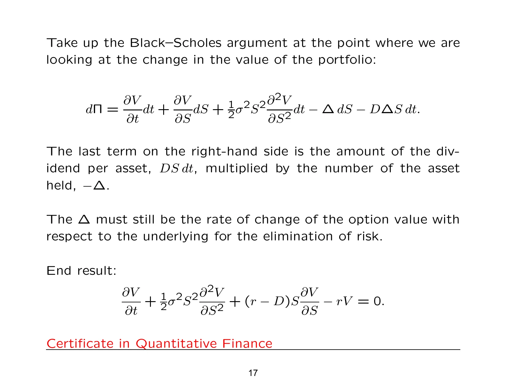
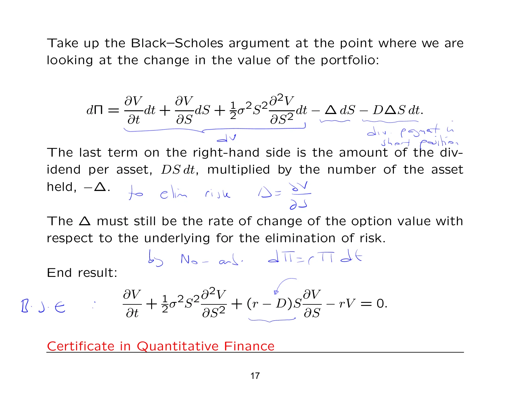
And that's what Paul's got over here. So this is dV, there's the minus delta dS, and this is the dividend payment in a short position, hence the minus. The next step is to eliminate risk. Set delta equal to dV by dS. You must have this. In an exam-type situation, if you don't have this wording, then you'd lose marks.
Then you would say, by no arbitrage, we have d pi equals r pi dt. Go through all the working, and then you end up with this. So when you have an option on an underlying which pays out a dividend, this is the Black-Scholes equation. However, if you were solving a real-life problem, then you wouldn't have this. What you'd have is extra jump conditionsjump conditions Jump conditions specify how a variable must behave when a process changes abruptly. to say what happens to S across the payment of a dividend. So there's the resulting equation.
Also, is it right to say that most functions will be parabolicparabolic Parabolic describes a class of partial differential equations with one time derivative and second-order derivatives in space. as we go up to the second derivative in the Taylor series, stroke Itô expansionItô expansion / Itô 4 Itô expansion is the stochastic-calculus analogue of Taylor series for functions of processes driven by randomness.? The parabolic comes from the balancing of dV by dt and the d-squared V by dS-squared term. That's where it comes from.
This is a slight extension. The mathematicians weren't particularly happy about the fact that you have this ideal assumption. But that said, there are a lot of stocks that don't pay a dividend. This is also an important equation that we're going to be looking at later on in terms of the solutions.
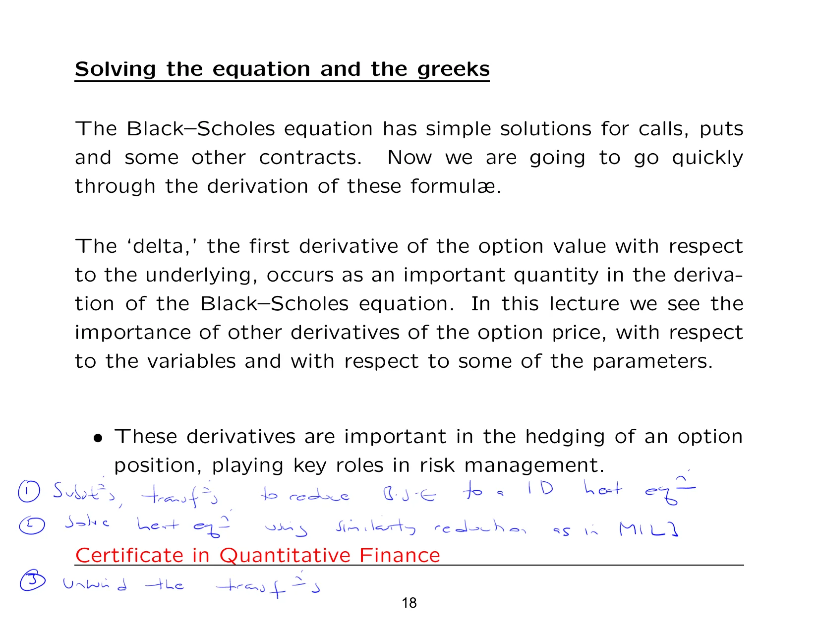
Now we come to the next bit: solving the equation and the Greeks. Solving the equation also consists of three parts. Part one: use substitutions and transformationssubstitutions and transformations Substitutions and transformations are algebraic or variable changes used to simplify a problem before solving it. to reduce the Black-Scholes equation to a one-dimensional heat equationheat equation / 1D heat equation The heat equation is a partial differential equation that models diffusion or heat flow in one spatial dimension.. That's the very first step. The second one is to solve the heat equation using similarity reductionsimilarity reduction Similarity reduction is a method for simplifying a problem by using a change of variables that exploits its scaling structure., as in Module 1, Lecture 3, the transition densitytransition density A transition density is the probability density of the future value of a process given its current state. stuff that we did. Step three is to unwind the transformations.
Now before we do that, I probably should write down the conditions. This is a partial differential equation, first order in time and second order in the underlying stock price. So we need three conditions. Let's write down call optioncall option A call option gives the holder the right, but not the obligation, to buy an asset at a fixed strike price. here, and on the other side we'll write down put optionput option A put option is a contract whose payoff increases when the underlying asset price falls below the strike price..
The first thing is our terminal conditionterminal condition / final condition A boundary condition specified at the final time, often equal to the option payoff at expiry., which is the payoffpayoff A payoff is the amount received from a contract at maturity, usually as a function of the underlying asset price.. So for the put, the payoff, which is our final condition, is going to be P(S,T) is max(E minus S, 0). This is a final condition, and the same goes here for the call.
Then we need a pair of boundary conditionsboundary conditions Boundary conditions are constraints imposed at the edges of a differential-equation problem.. When S becomes very small, then C is worthless. When S becomes very large, then C behaves like S; it's about the same size. In the case of a put optionput option A put option is a contract whose payoff increases when the underlying asset price falls below the strike price., when S becomes very large, then P vanishes. And when S is zero, use the put-call parityput-call parity Put-call parity is the relationship between the prices of a put and a call with the same strike and expiration.: C minus P is S minus the discounted strike pricestrike price / strike The strike price is the contract price used to exercise an option, also called the strike.. We know that when S is zero, C is zero, so P then becomes the discounted strike pricediscounted strike price The strike price after discounting it back to present value..
So six conditions in all, three for each option. The Black-Scholes equation, or any equation, needs to know what the conditions are for a particular type of product in order for it to price it. Any questions on that? No, because it is all maths really.
So here's the Black-Scholes equation. Let's start with step one. Step one is to use transformations and substitutions, which are motivated by both financial and mathematical ideas. As long as they make sense, we can use them. The first thing is to write down the price of the option as the present valuepresent value Present value is the value today of a future cash flow after discounting. of some unknown function, which is what you see next to the bullet point. V is the present value of some u.
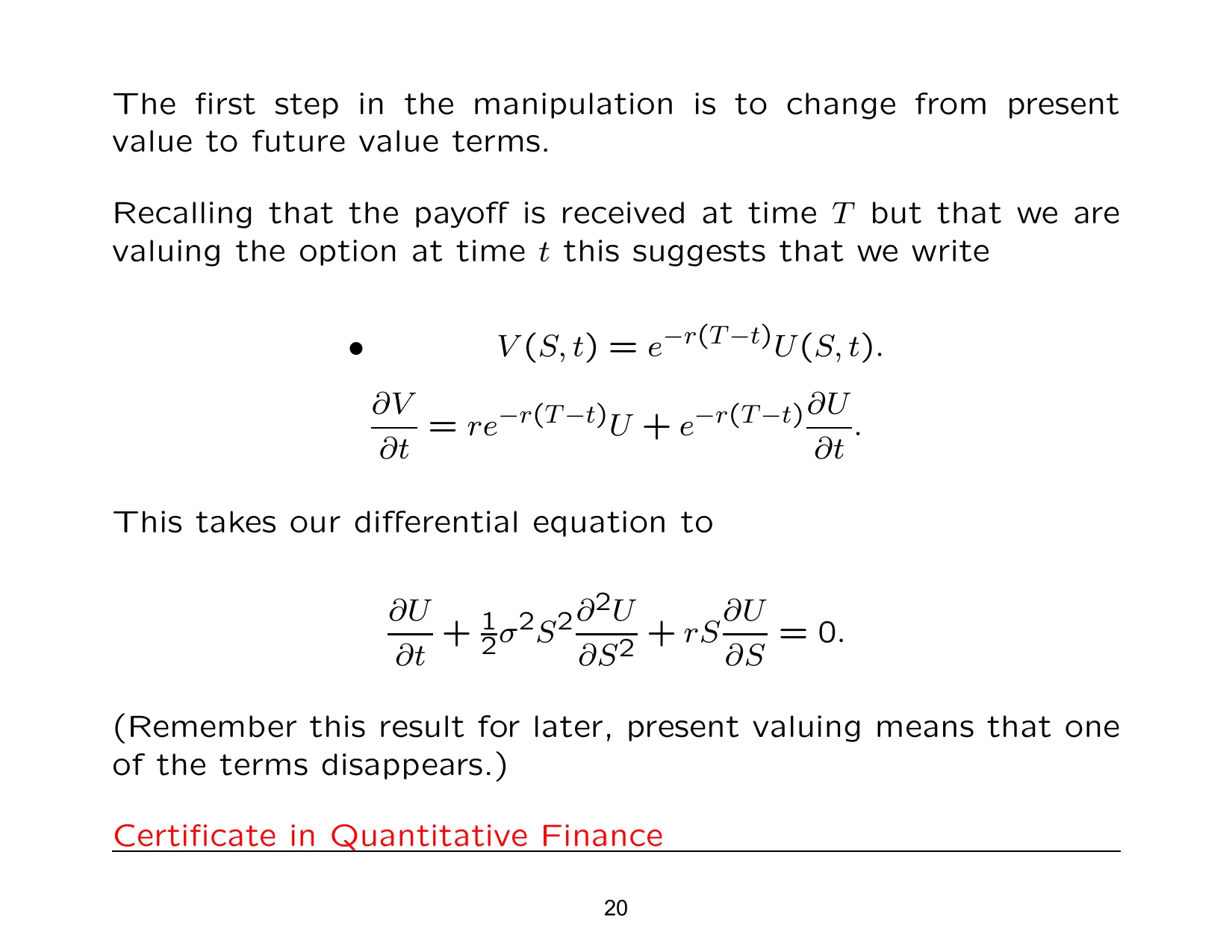
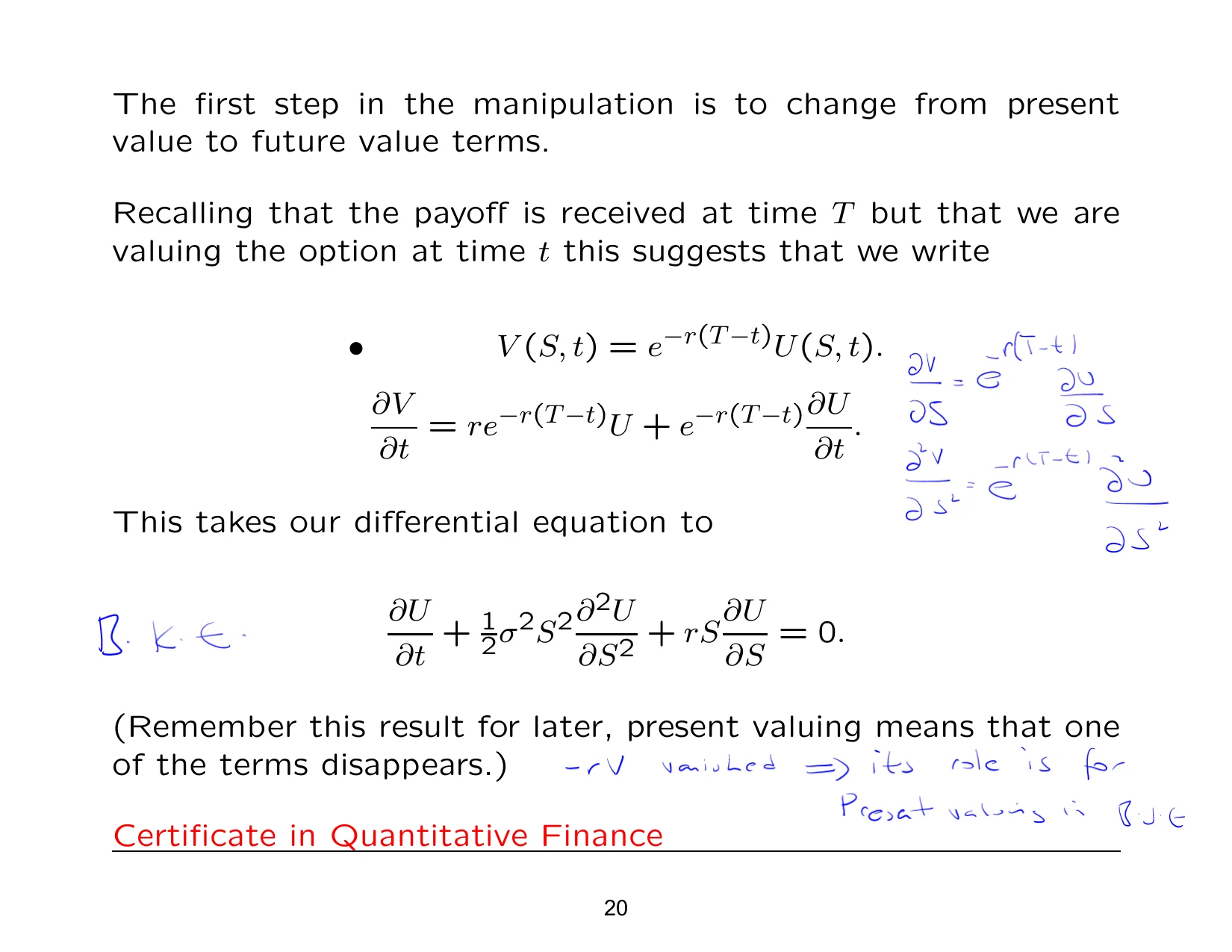
We can also write down what dV by dS is, and then d-squared V by dS-squared is e to the minus r times T minus t, d-squared u by dS-squared. We substitute those into the Black-Scholes equation, and what we're left with is this. This is the backward Kolmogorov equationbackward Kolmogorov equation The backward Kolmogorov equation is a PDE for the expected future value of a stochastic process, written backward in time.. What do you notice? The minus rV has vanished, which implies that the role it performs is present valuing in the Black-Scholes equation.
Step two is to write down the time, rather than having t, in terms of the time to expirytime to expiry Time to expiry is the amount of time remaining until a contract or option expires., which means we can now say that d by dt becomes d by d tau, but then we have to use a chain rule here, so it becomes minus d by d tau.
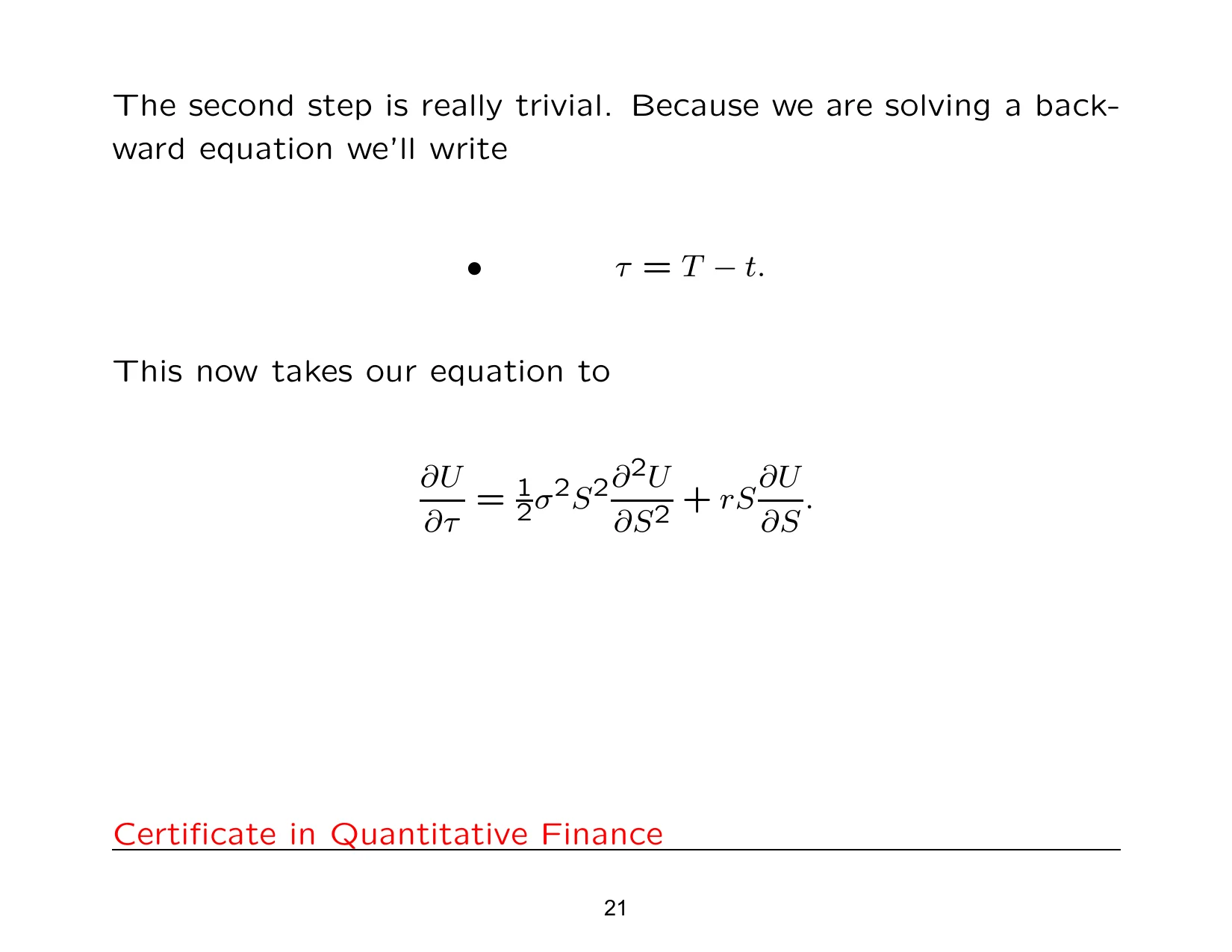
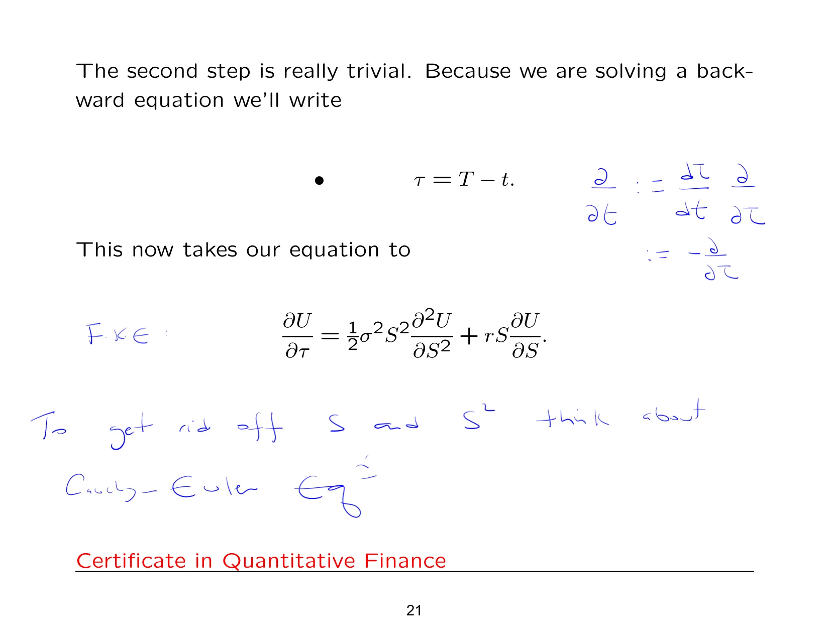
This means we can now say that d/dt becomes d/dtau, but then we have to use a chain rule here, so it becomes minus d/dtau. The minus comes in, so we can take that time derivative term onto the other side, and it starts to look a bit more like a heat equationheat equation / 1D heat equation The heat equation is a partial differential equation that models diffusion or heat flow in one spatial dimension.. And this is the forward Kolmogorov equationforward Kolmogorov equation An equation that governs the time evolution of a process’s probability density..
If we're going to make it look like a heat equation, we have to get rid of those variables s and s squared. To get rid of s and s squared, think about the Cauchy-Euler equationCauchy-Euler equation The Cauchy-Euler equation is a type of differential equation with coefficients that scale with the variable.. As a hint, this is the Cauchy-Euler equation, which means using a log transformationlog transformation / log of the price A log transformation rewrites the price in logarithmic form so that changes are handled additively instead of multiplicatively.. And that's the next step: let xi equal log of s.
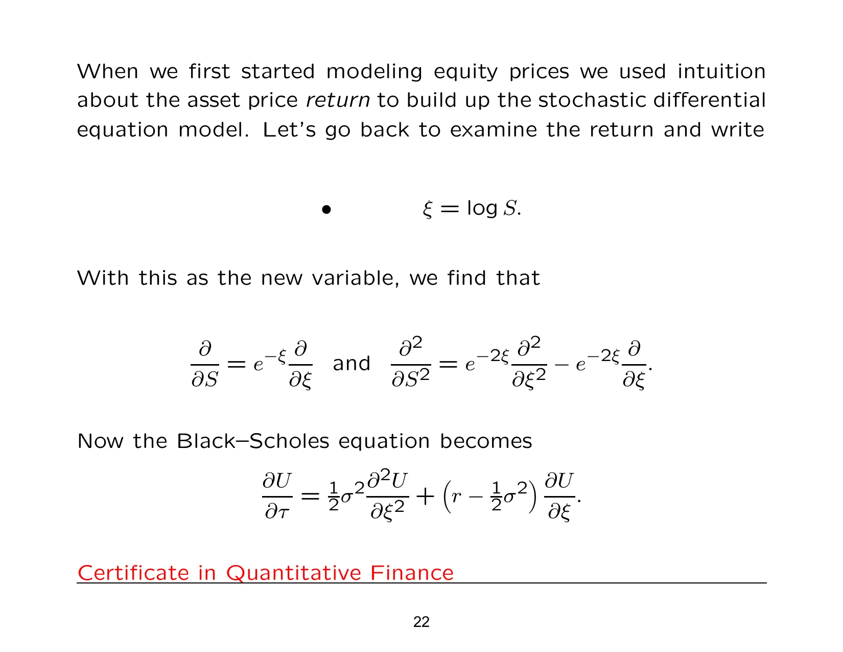
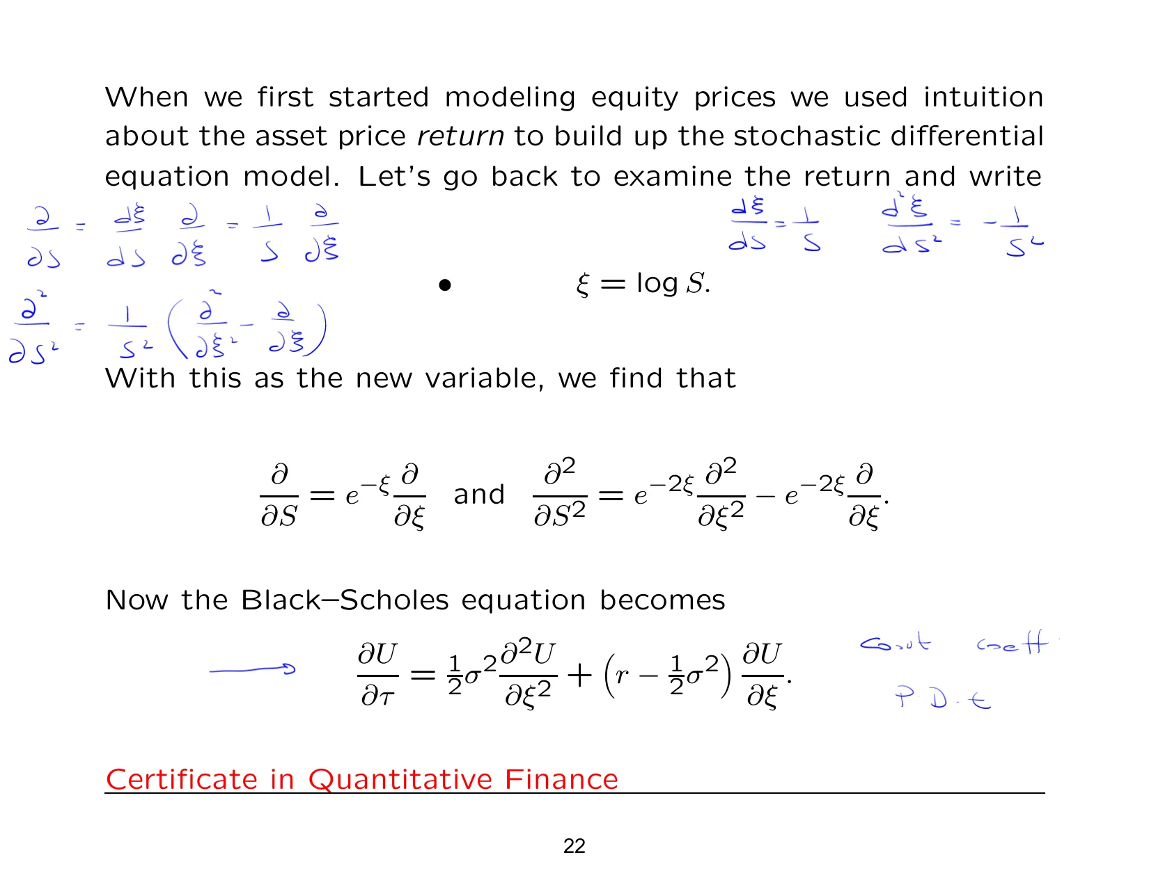
So now let's work in terms of the log of the pricelog transformation / log of the price A log transformation rewrites the price in logarithmic form so that changes are handled additively instead of multiplicatively.. We need these, and we can then say that d/ds becomes 1/s d/dxi. If you carry on working like this, you'll then find that d squared by ds squared is in fact 1 over s squared times d squared by dxi squared minus d by dxi. Those are the transformations you now need, and when you substitute this into the equation on the previous slide, you'll find that the s and the s squared cancel out.
We're now left with a constant coefficient partial differential equationconstant coefficient partial differential equation A constant coefficient partial differential equation is a PDE whose coefficients are constant rather than variable.. The last step specifies a translation of the coordinate system. The extra notes that you're going to have will show you how to use chain rule 2, chain rule 2 for partial derivatives. After you substitute this in, you're left with this, and that's the 1D heat equation.
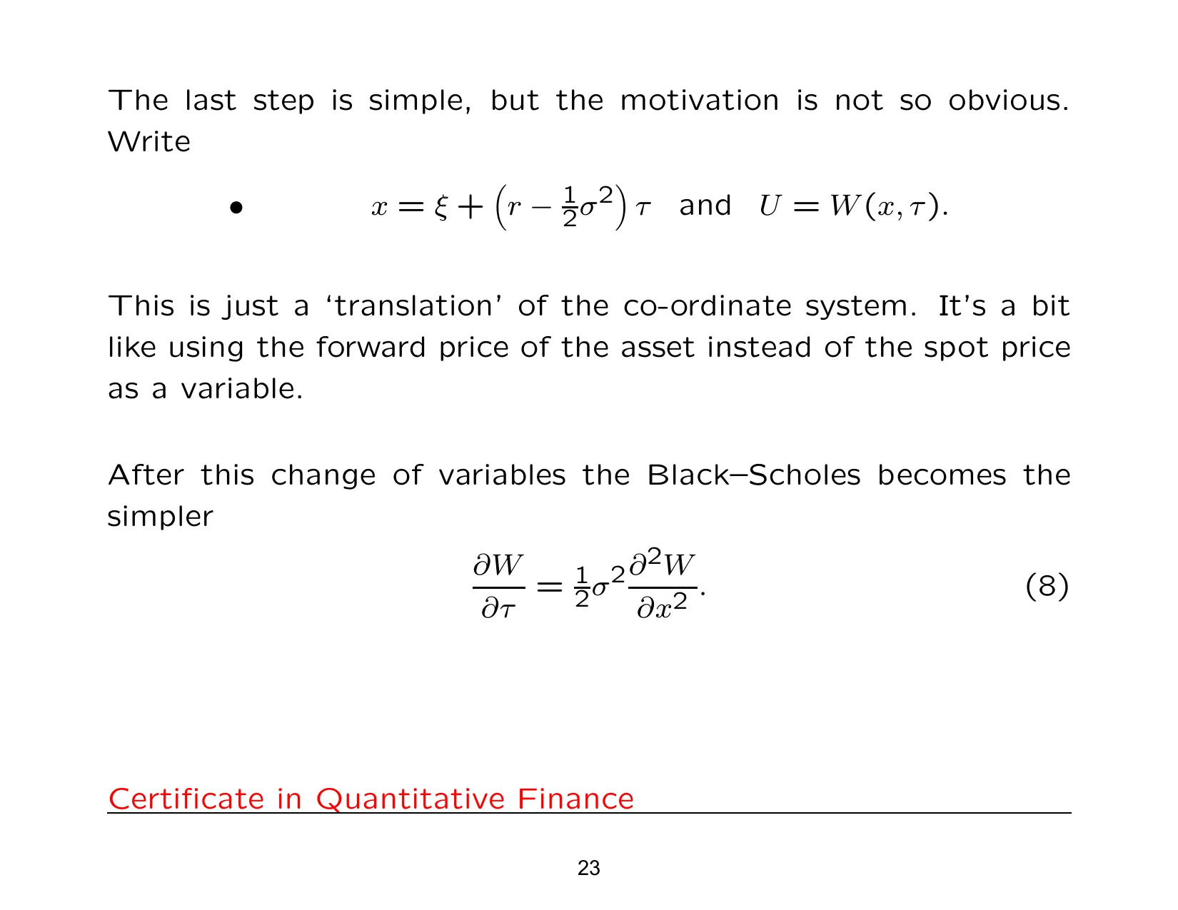
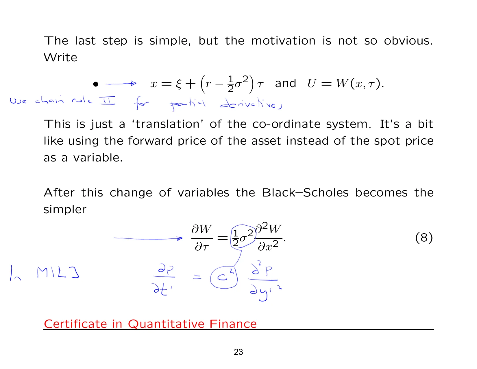
Now when you look at equation 8, do you recognize something interesting about it? If you remember in module 1, lecture 3, we said that later on this is going to be replaced by the volatility of the stock. So in other words, we've got the variance there. Remember that equation, because later on you're going to see that. And the c squared will be related to c squared there, where c was some generic universal constant.
Now we're working in finance, so you can actually see things from finance making their presence known. What's the good news? This is good news. Paul says we've seen this before, and we've solved it using similarity reductionsimilarity reduction Similarity reduction is a method for simplifying a problem by using a change of variables that exploits its scaling structure., which means you don't have to do that again. In hindsight, if you think back to module 1 and it was a painful experience, the good news now is we don't have to do any of that, because you've seen how to solve this using similarity reduction. What we're more interested in now is the application to quantitative finance.
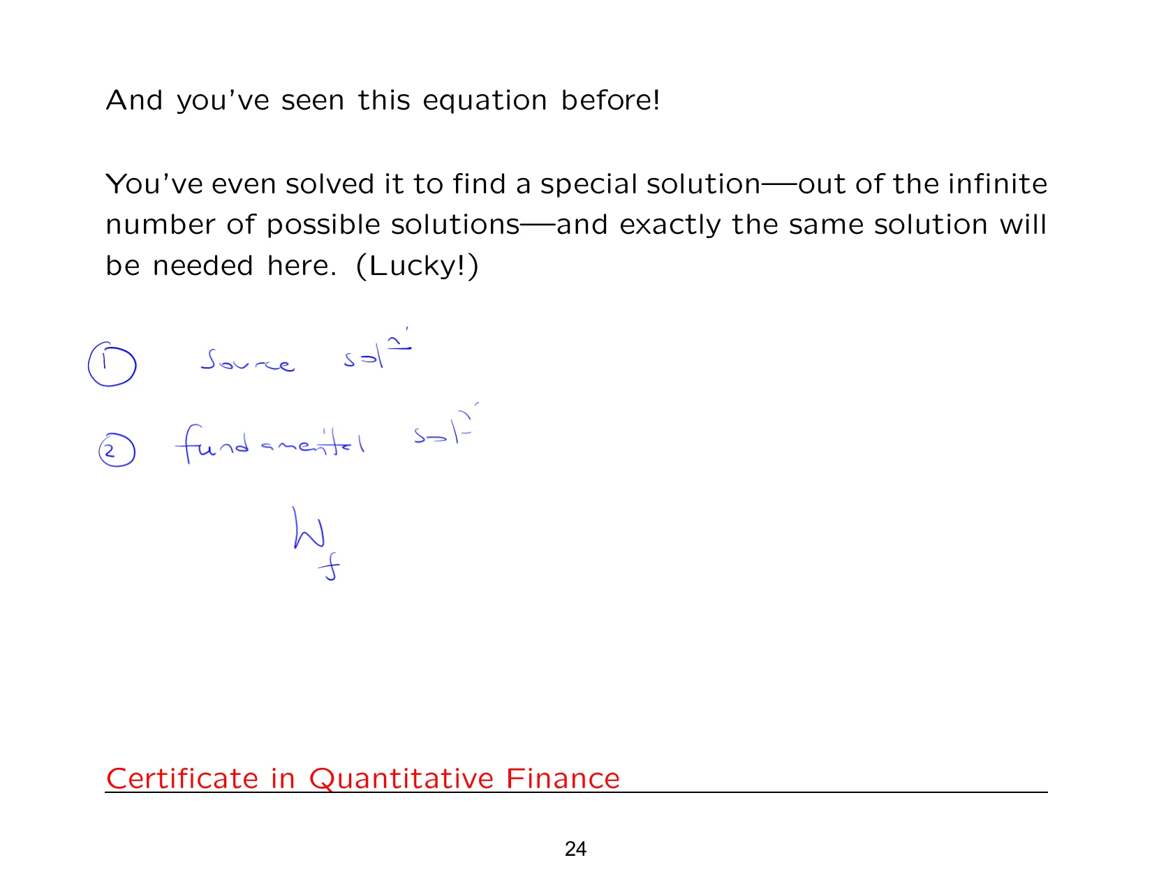
That special solution that we saw earlier on has two names that we used in module 1, lecture 3. You could call it the source solutionfundamental solution A solution of a PDE corresponding to a point source, often used as a building block for other solutions. or the fundamental solution, often written down as W_F. This is a summary of all the transformations that have been done. You start off with this, this is the starting point, and you reduce it down to a problem which is essentially the present valuepresent value Present value is the value today of a future cash flow after discounting. of this function W.
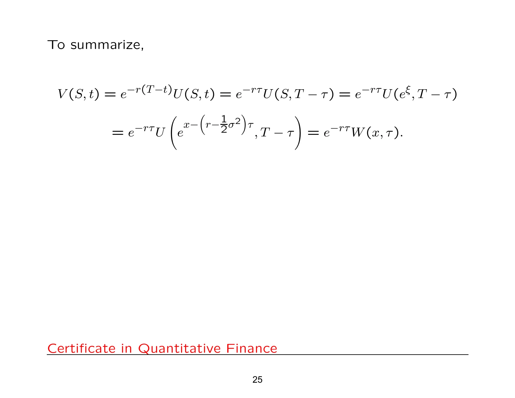
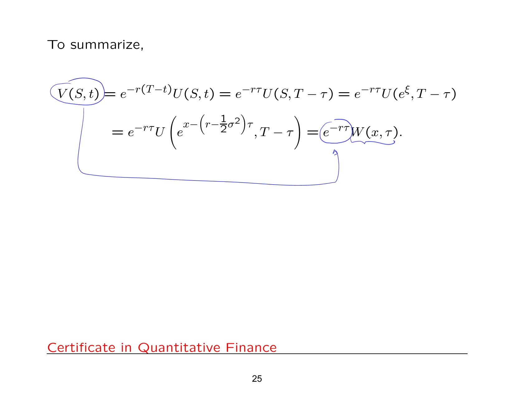
Obviously, once you've solved this, then there's going to be quite a lot of messy work in going backwards. But this is a summary of all the transformations that have been done. So we're going to look at plain vanillas. Paul says the first step is to find that special solution; we know how to do that. Remember when we solved it before, normally all you'd have is something like a 1 over root t, and then some function of x over the square root of t.
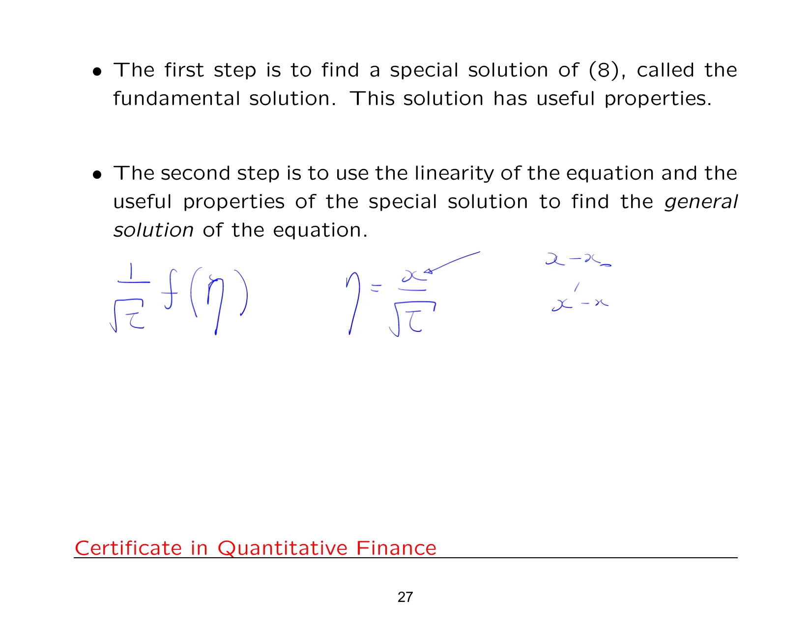
Let's get rid of that, because that's what we used last time. What this did was give it a mean of zero. You can center it about some non-arbitrary, non-zero value, so you could have something like x minus x naught, for example, or you could have x prime minus x, which is what Paul does over here. And when you do the same working with that starting solution, this is what you end up with. Remember before we had a c squared there; now we've got a sigma squared here. We've got a tau here, the time.
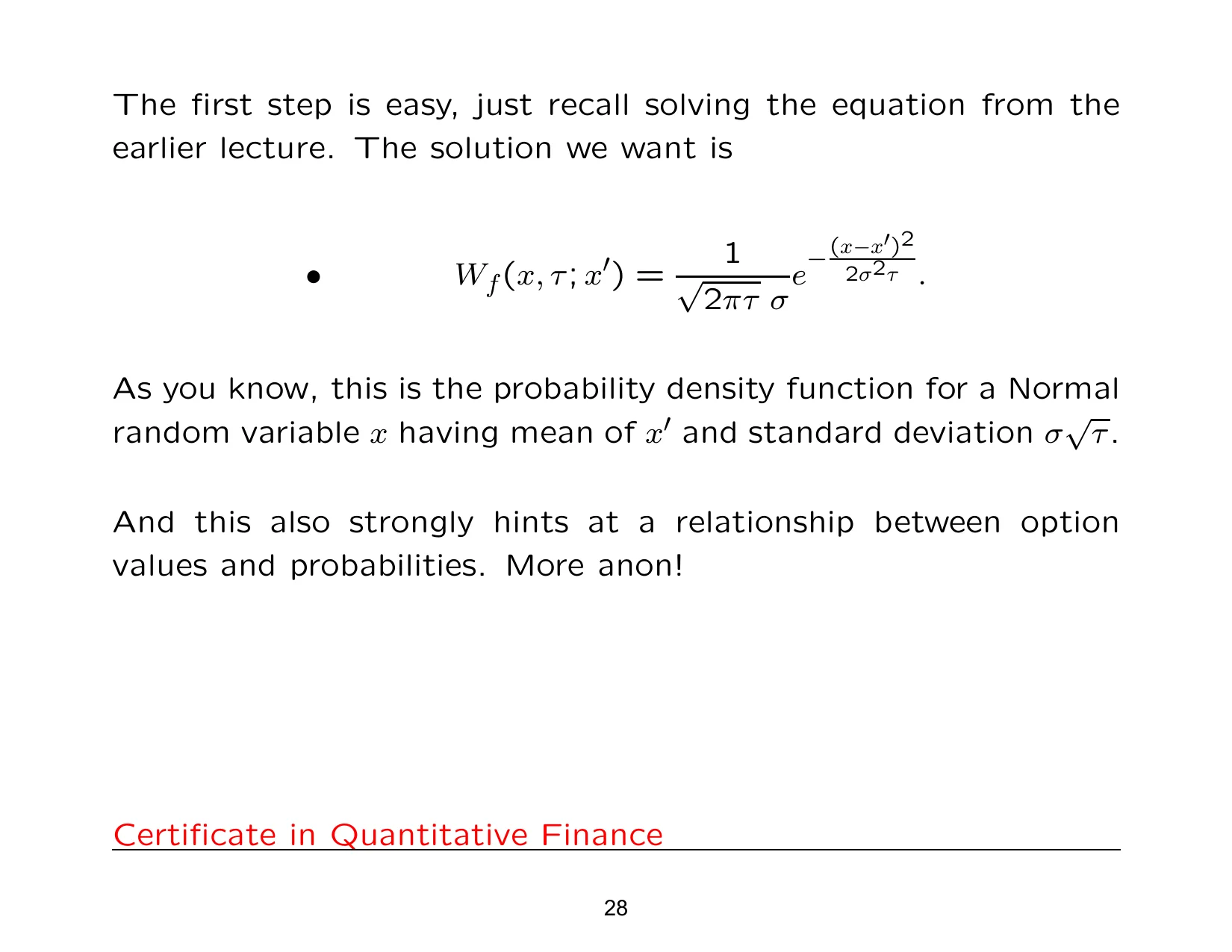
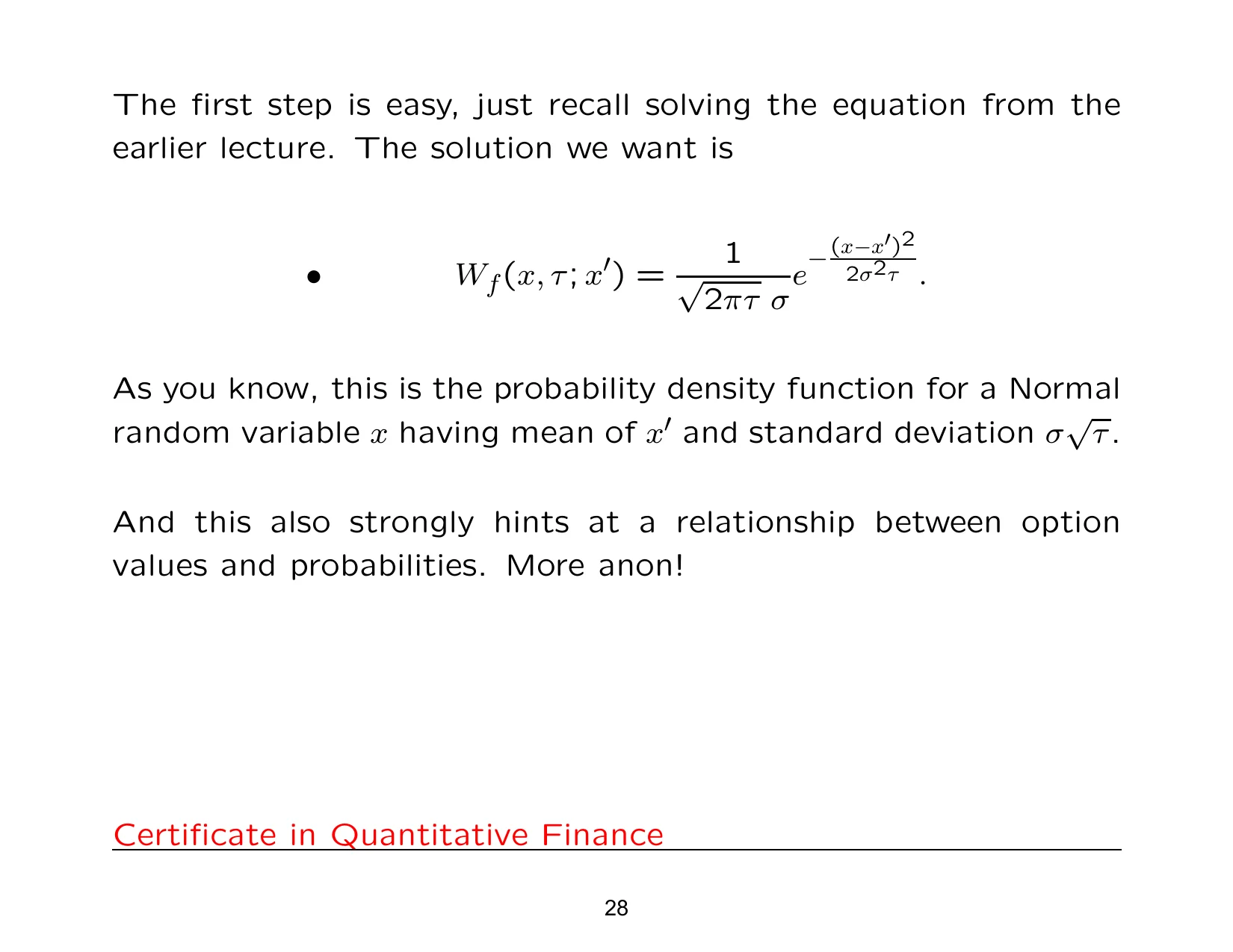
The good thing is we're not going to go through all that working again, because we spent almost an hour on this in module 1. We're certainly not going to waste another hour looking at the solution method, because you've all done that. I'm going by a lot of the questions I've been getting on Helpdesk. A lot of you have been working through this.
Remember that graph from last time? We started with a spike. In other words, right at the beginning we've got this singular behavior over here, zero on either side, and this is how it diffuses out. We also mentioned the term Dirac delta functionDirac delta function An idealized distribution concentrated at a single point, used to model impulses and point sources.. Again, you don't really need to know about the Dirac delta function, because we can still do everything that we need to do this evening without you really knowing too much about its mathematics.
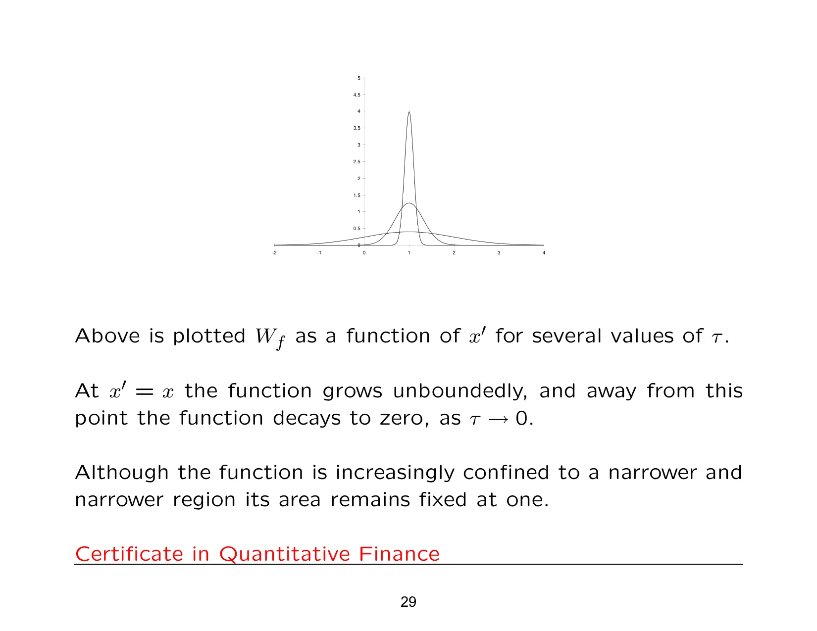
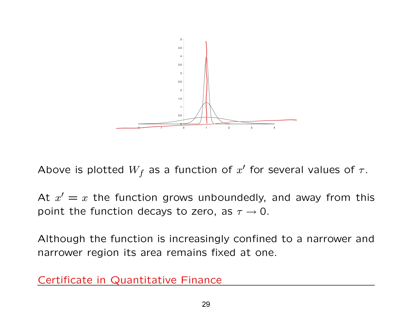
It's just a certain type of behavior when the tau becomes very, very small. And then there are all sorts of properties: differential properties, integral properties, of a Dirac delta functionDirac delta function An idealized distribution concentrated at a single point, used to model impulses and point sources.. So we can bypass this and go straight down to this page here, fortunately. This is where we pick up, and fortunately for us, Paul says, I'm now going to cut to the chase and simply quote this result here.
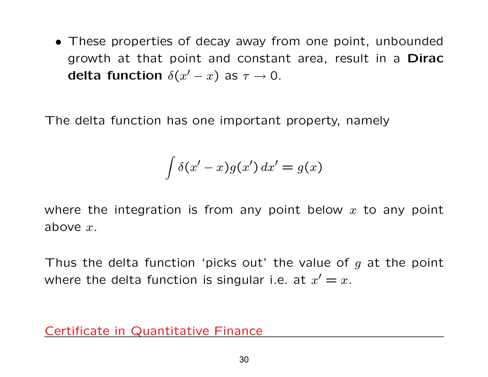
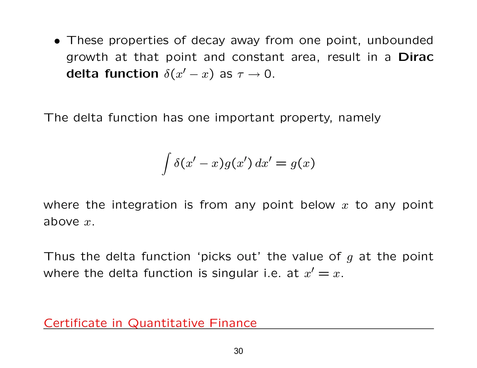
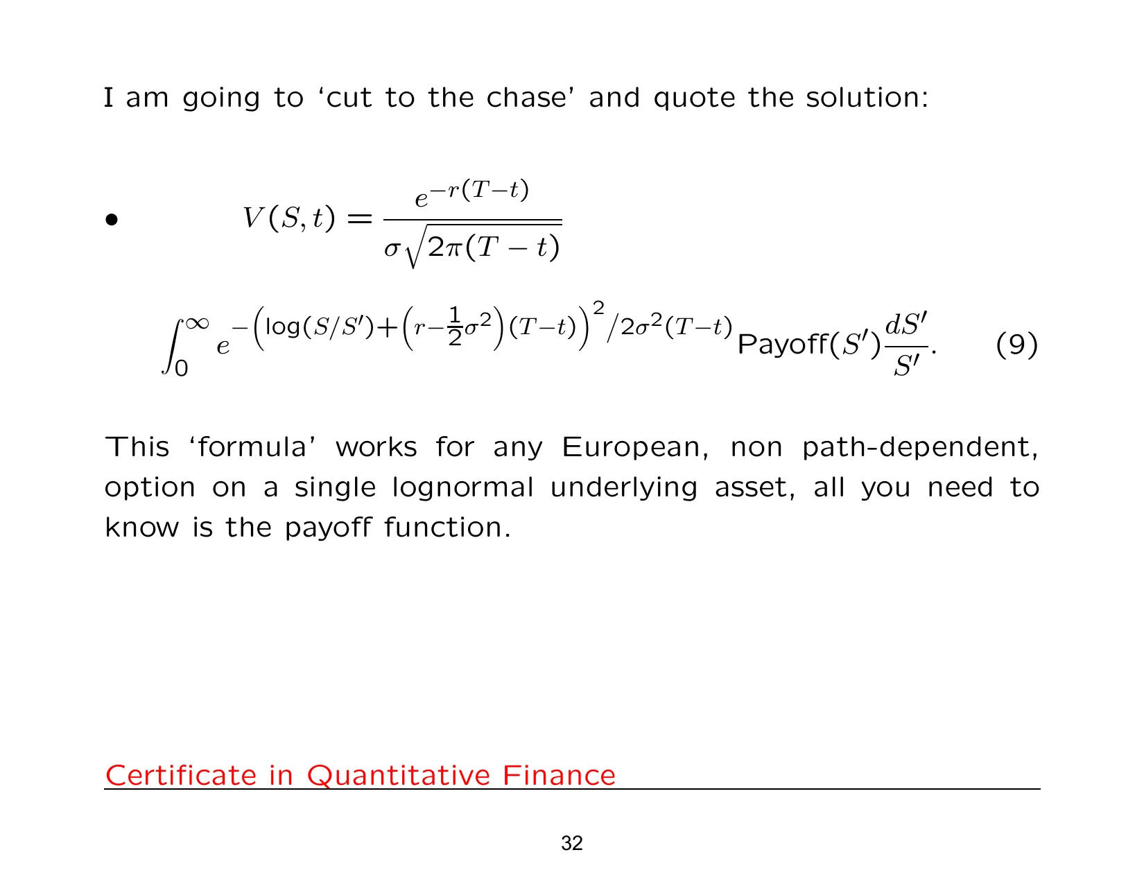
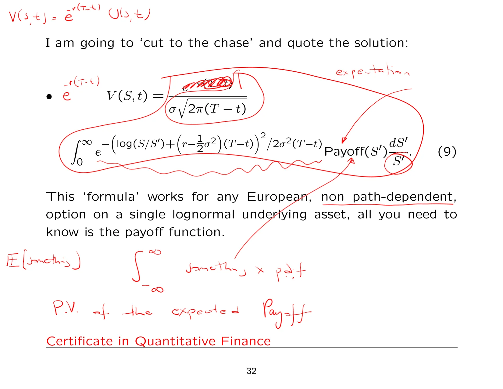
Let's remind ourselves of step one. Remember step one was this. What that tells us is that, if I take this to the other side, u is this very, very messy-looking long expression. So it's a good thing to now try and interpret this.
If we try and interpret this, what is this? We know that the exponential is the present value term, and then we've got this thing here. That tells us that all of this is an expectation. And remember, what does an expectation comprise? You integrate from minus infinity to plus infinity. If I had the expectation of something, I'd integrate it between minus infinity and plus infinity, take the something, and multiply it by its PDFPDF / probability density function PDF stands for probability density function, the function that describes the density of probability for a continuous random variable..
Now what's the something over here? A payoffpayoff A payoff is the amount received from a contract at maturity, usually as a function of the underlying asset price.. So we can see that it's some kind of expectation of a payoff, which means that everything else, meaning this term here and all of that, that term and the one over this, that's our transition density function for a stock price. That's where it comes from.
Equation nine is the present value of the expected payoffpresent value of the expected payoff The present value of the expected payoff is the discounted current value of the payoff averaged over its probability distribution.. Would you agree? It also tells us exactly what the transition density for a stock price is. It's the one over sigma square-rooted times an s prime times the exponential, so present value of the expected payoff.
Obviously, there are tons and tons of lines of working missing here, which you're going to capture, or you're going to see, in my extra typed-up notes. Even to get from the previous slides to here, there are quite a few steps missing, because there have been quite a few transformations unwinding. And what's basically going to happen now is that you have to do a lot of integration by substitution and get some really messy terms for the limits of integration.
Any questions or thoughts on this? Everyone happy?
What's basically going to happen now is that you have to do a lot of integration by substitution and get some really messy terms for the limits of integration. Any questions or thoughts on this? Everyone happy? Let's scroll down then.
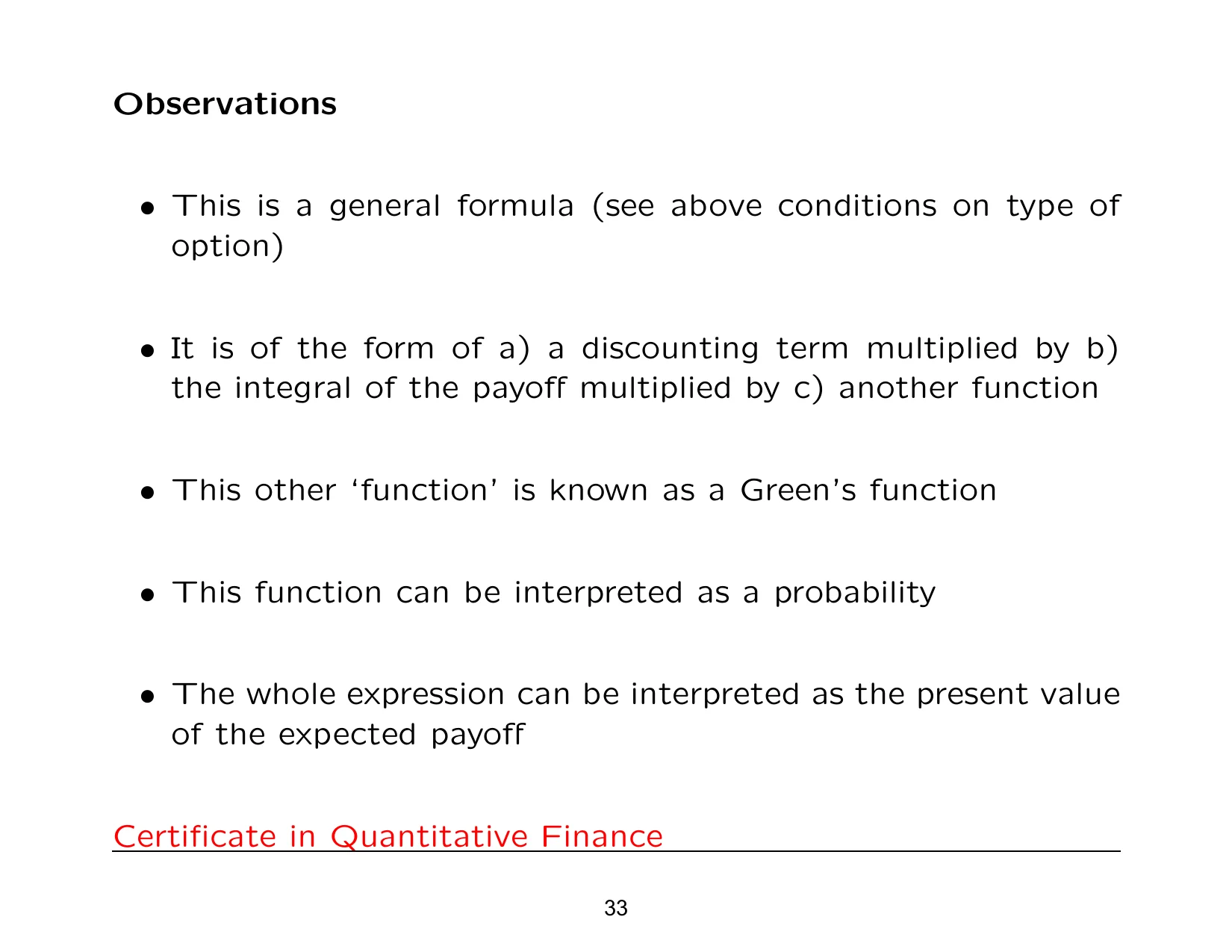
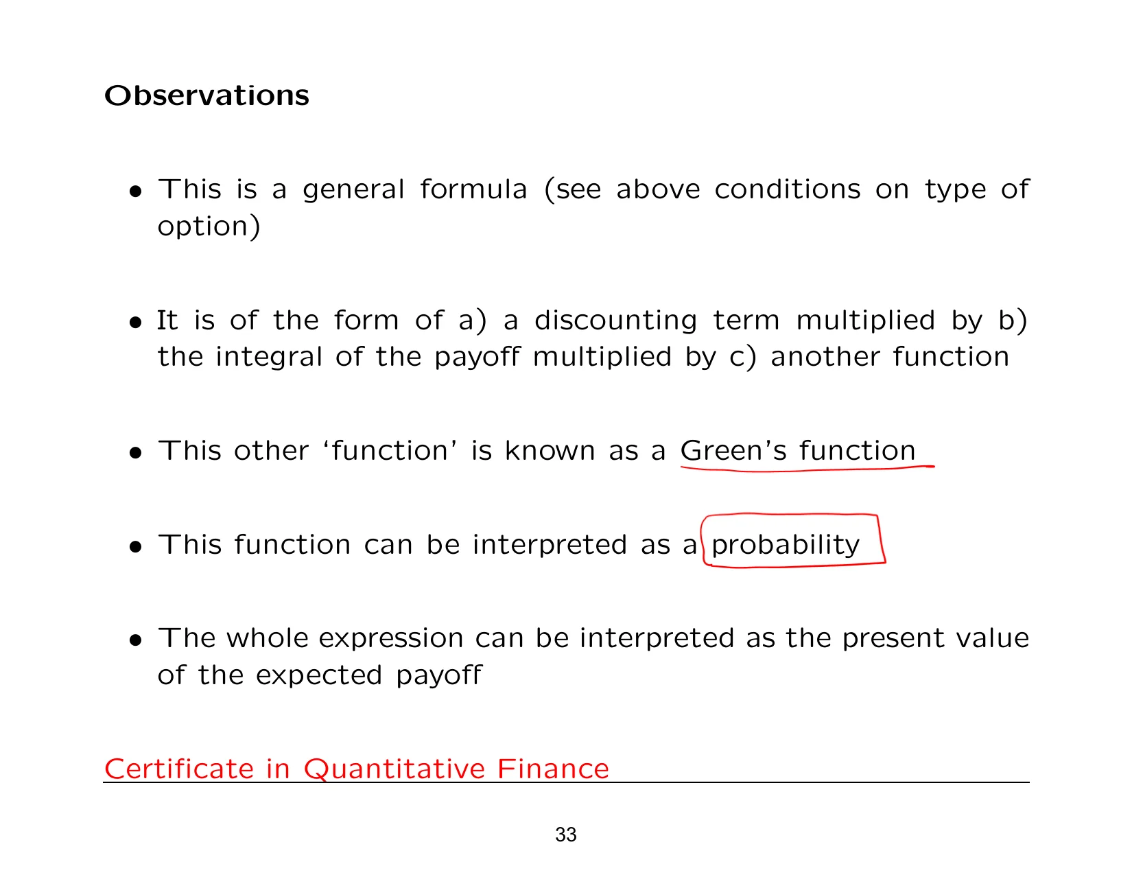
These are the properties of equation nine. It says this is a general formula. Why is it general? Because it just says payoff. It doesn't actually specify what kind of payoff. So expression nine has no idea what kind of payoff or option it's trying to price.
It comprises three bits. There's a discounting term, which I took to the other side just because I wanted to focus on what was left over. There's an integral of the payoff, and then there's this long messy function that's multiplying with that.
The other long messy function has two names. If you're in the business of solving partial differential equations as a branch of maths, then it would be called a Green's functionGreen's function A function used to represent the response of a linear PDE to a point source or impulse.. If you're working in quantum finance or you're working in probability theory, then it's a PDFPDF / probability density function PDF stands for probability density function, the function that describes the density of probability for a continuous random variable.. We're more interested in the fact that the one over sigma square root term times that exponential is the transition PDF.
Multiplying the transition PDF with the payoff, then integrating between minus infinity and plus infinity. Remember, stock prices can't become negative, so we go from zero to infinity rather than from minus infinity to zero and then zero to infinity. That wouldn't make sense. When we express this collectively, we've got the present value of the expected payoffpresent value of the expected payoff The present value of the expected payoff is the discounted current value of the payoff averaged over its probability distribution..
As I said, remember, there's a lot of fiddly working that goes into this. So now let's look at special cases, that is, define a particular payoff.
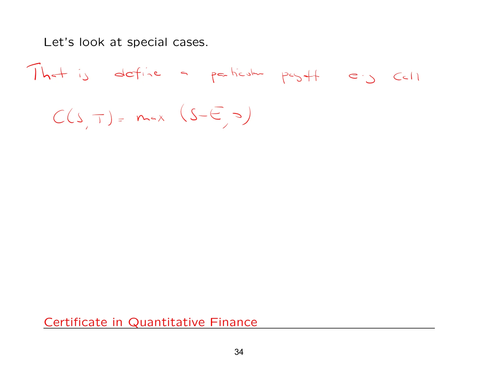
There is something important I need to tell you. The reason why this works is because it's a European payoffEuropean payoff A payoff determined only at maturity, as in a European-style option., in other words, a European call optioncall option A call option gives the holder the right, but not the obligation, to buy an asset at a fixed strike price.. It's path independentpath independent Path independent means the result depends only on the starting and ending points, not on the path taken between them., so we can simply take the final conditionterminal condition / final condition A boundary condition specified at the final time, often equal to the option payoff at expiry., put it in here, and then integrate it. Normally, you put an initial condition. Remember, in quant finance and derivative pricingderivative pricing The process of valuing a derivative contract using a mathematical or financial model., we have final conditions from which we can work out the solution earlier, and that's how Green's functionGreen's function A function used to represent the response of a linear PDE to a point source or impulse. works.
If you've done PDEs in a bit more of a theoretical framework, you'll appreciate exactly what this means. So here's the payoff for a call option. Remember, we want to be in the moneyin the money An option state where exercising the contract would produce positive intrinsic value., so we go from E to infinity because from zero to E that's going to be zero, so we can just go from E to infinity. There's the payoff.
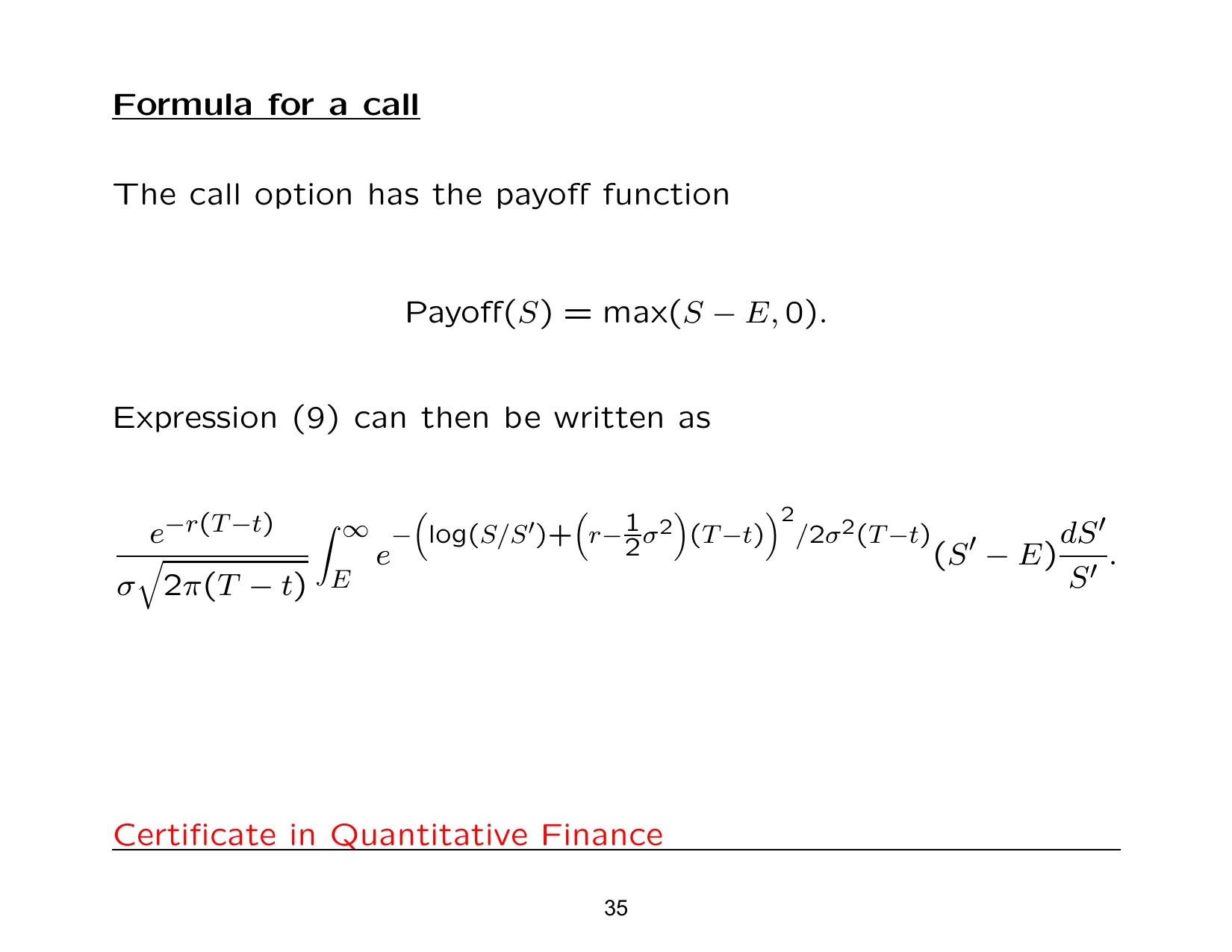
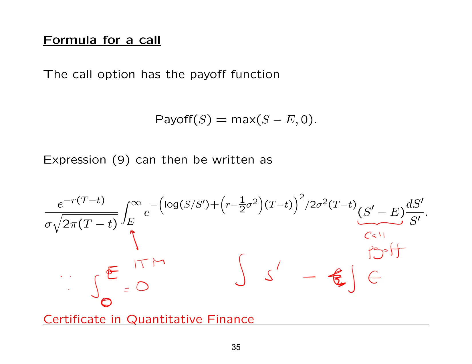
So we're going to have two integrals here. We're going to split this up into two integrals, one with S prime in it, minus E times some other integral. So it's going to decompose into two integrals. Probability interpretation: a probability of being in the moneyin the money An option state where exercising the contract would produce positive intrinsic value..
Not so much profit, but we'd say being in the money, because this is from the view of the holder. How can this factor come before? Have a serious think. Can we pull out a constant out of an integral? Yes or no? E is a number. S prime is inside the integral. E has been pulled out. But if it's going to cause a lot of stress, just put it back in. There we go. No big deal.
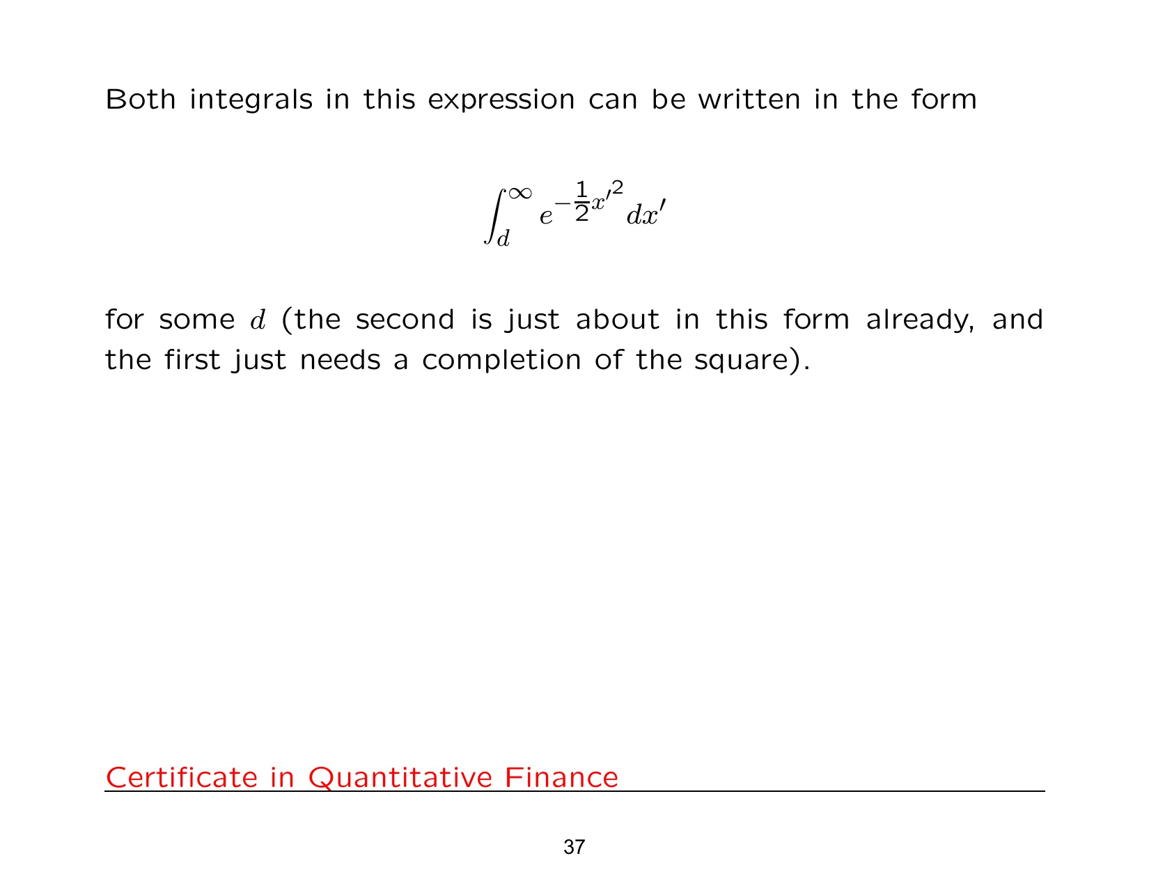
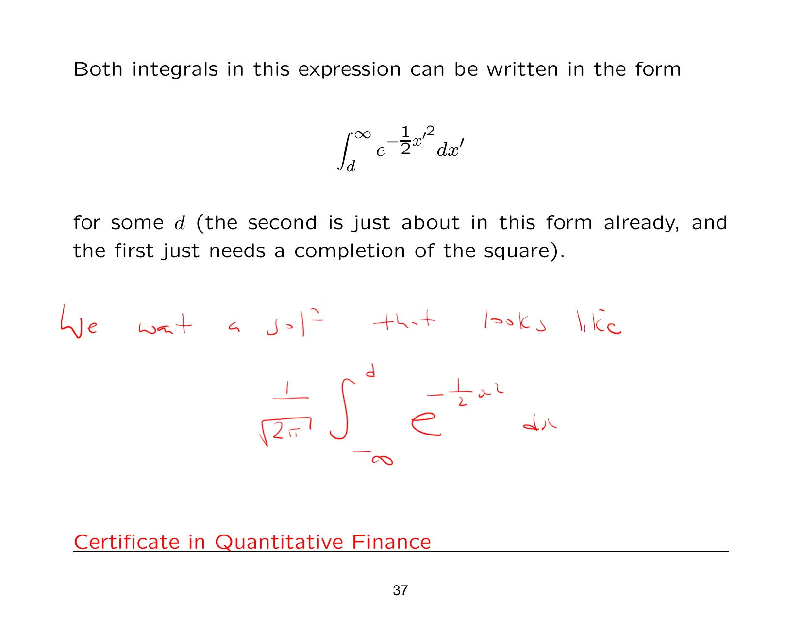
So here's the next couple of steps, plus much messy working, a lot of messy working. After we've done all of that, the idea is to try and write this down in terms of the cumulative distribution functioncumulative distribution function CDF stands for cumulative distribution function, the function that gives P(X ≤ x) for a random variable X.. So we want a solution that looks like the following: it goes from minus infinity to some value over here, d, with a 1 over root 2 pi outside, and also e to the minus a half x squared dx. So we can write it down in terms of the cumulative distribution function for the normal distributionnormal distribution The normal distribution is a symmetric bell-shaped distribution characterized by its mean and variance..
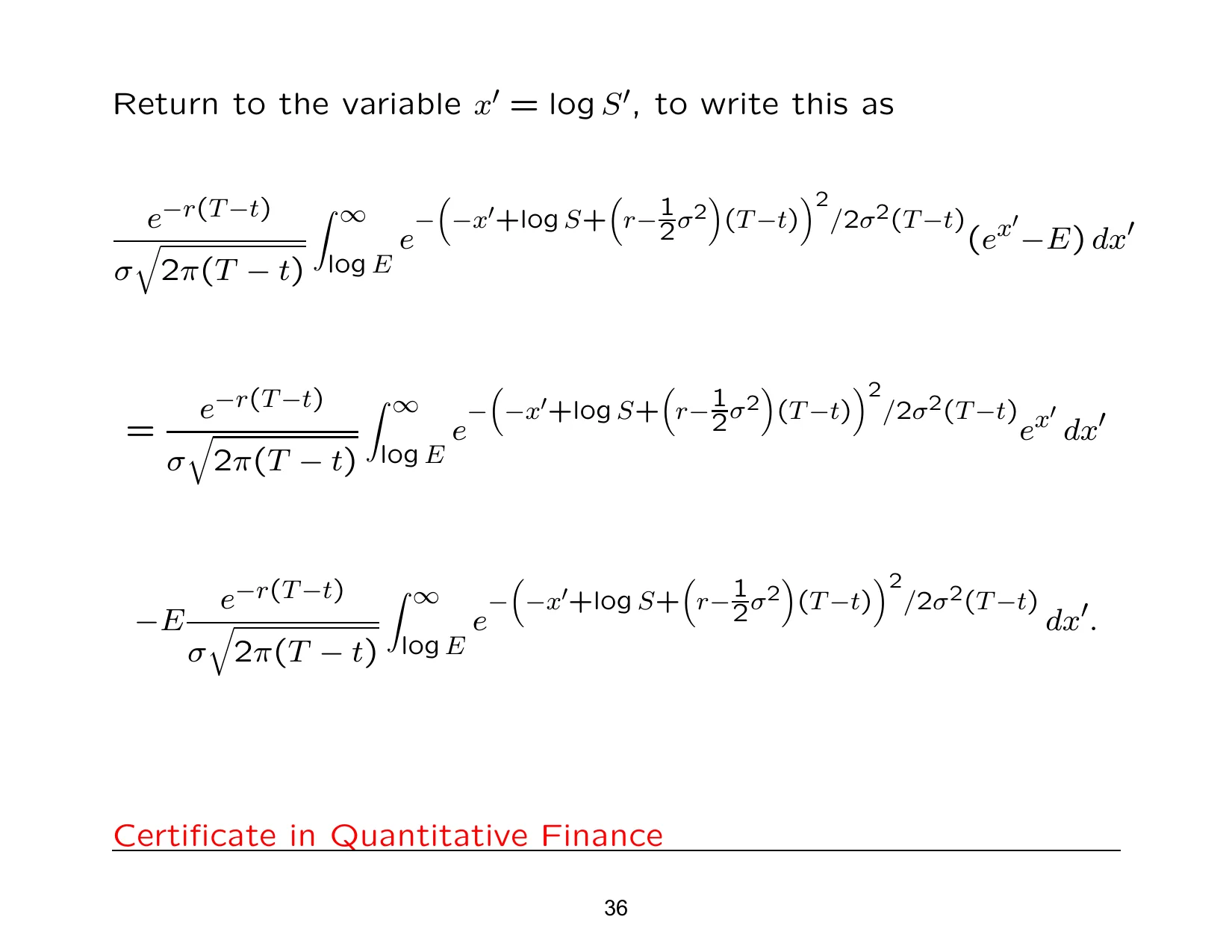
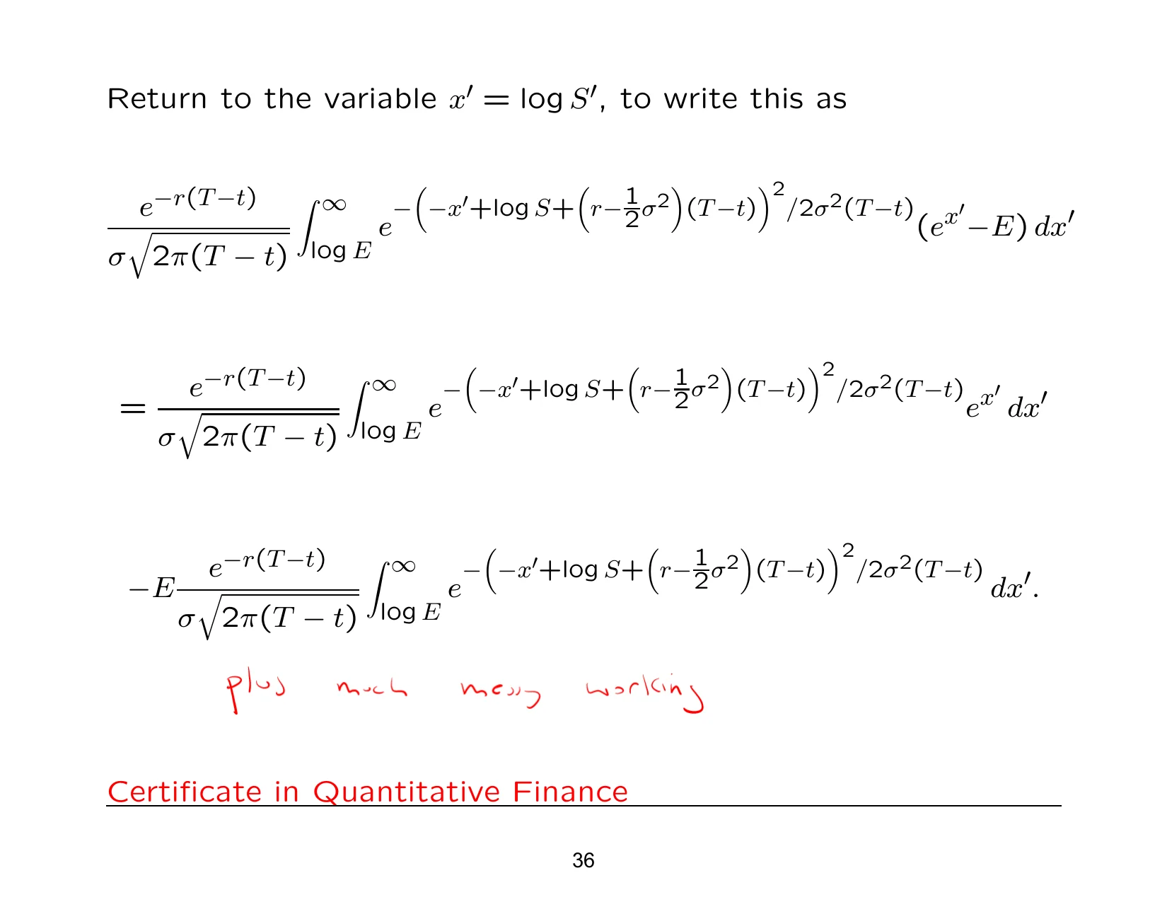
After we've done all that working, this is what it ends up with: S N(d1d1 and d2 d1 and d2 are the two standard intermediate quantities that appear in the Black-Scholes pricing formula.) minus this.
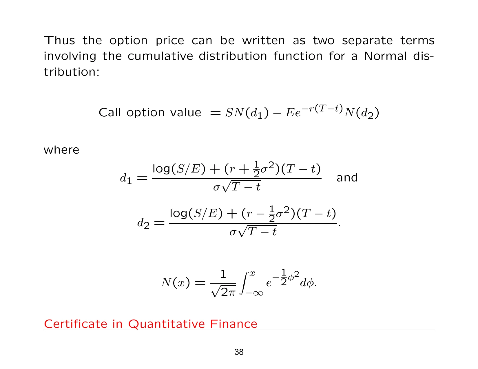
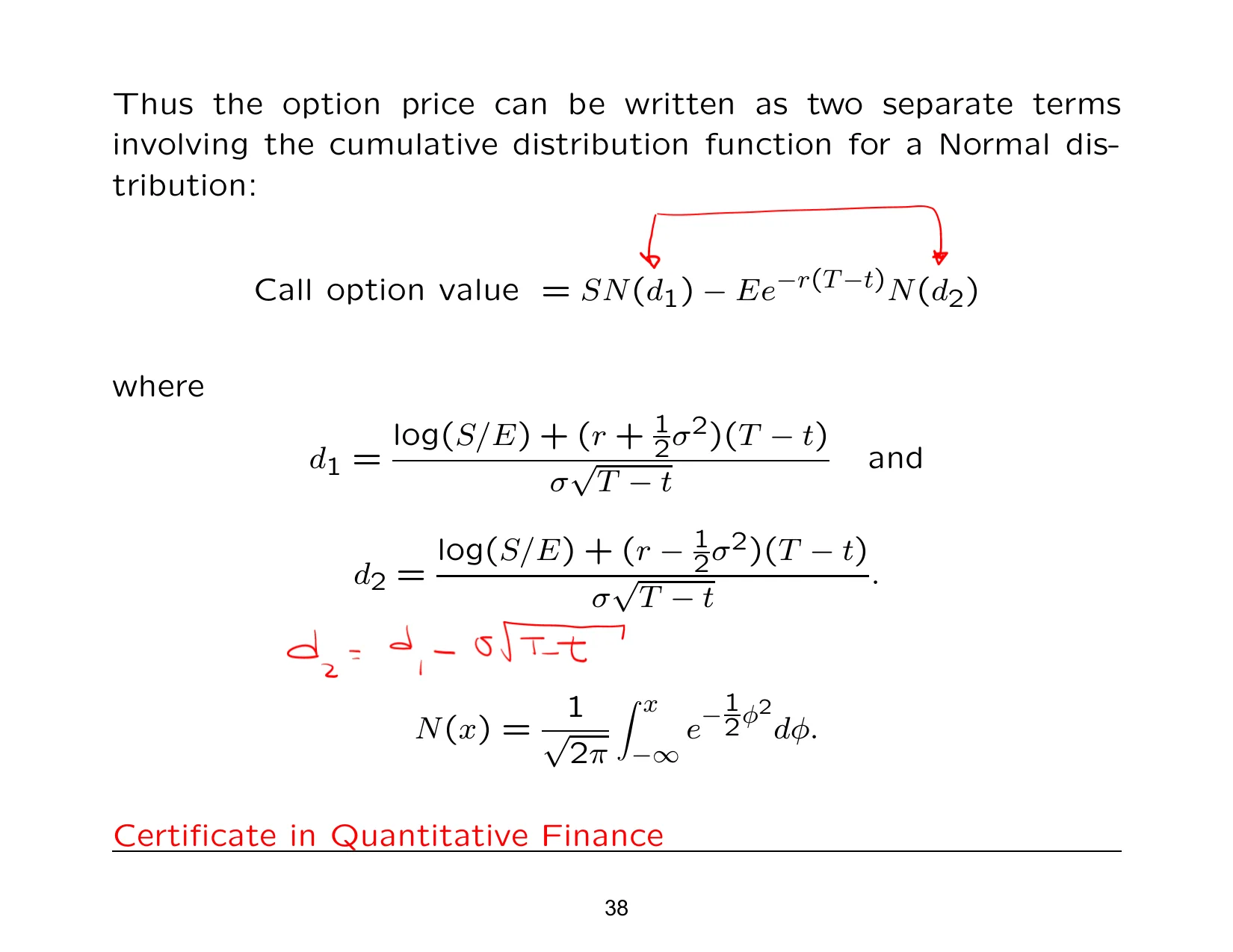
Now there's been a lot of confusion over the years. People tried to interpret d1 and d2d1 and d2 d1 and d2 are the two standard intermediate quantities that appear in the Black-Scholes pricing formula., and in the last cohort what I did was I found an article where someone had interpreted d1 and d2 to make it look more logical. I don't know if that's on the portal. It may be, and that way you can see exactly what the interpretations of d1 and d2 are.
d1 is normally regarded as a bit more intuitive than d2, but someone actually wrote an article to explain this because the mathematicians didn't worry too much about trying to interpret d1 and d2 in financial terms or in physical terms. That's the price of the option, and d1 and d2 are linked together. d2 is written down as d1 minus sigma times the square root of t minus little t.
Whether it's in the money, out of the money, or at the moneyat the money At the money means an option’s strike price is equal, or nearly equal, to the underlying asset price., when you have a look at that article it'll explain. That was after a few years of people asking me to interpret that, so I thought, let me see if I can find something. The only place I found a useful interpretation was that particular article.
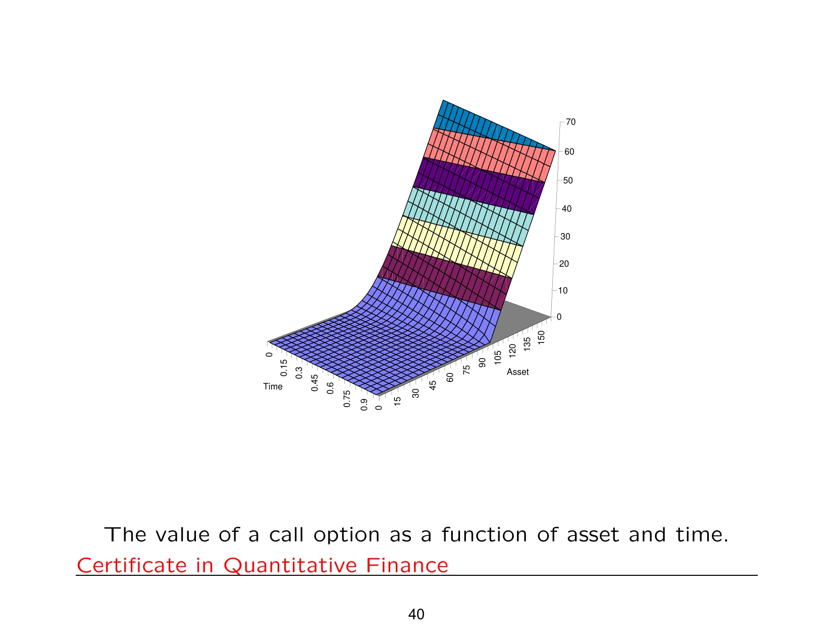
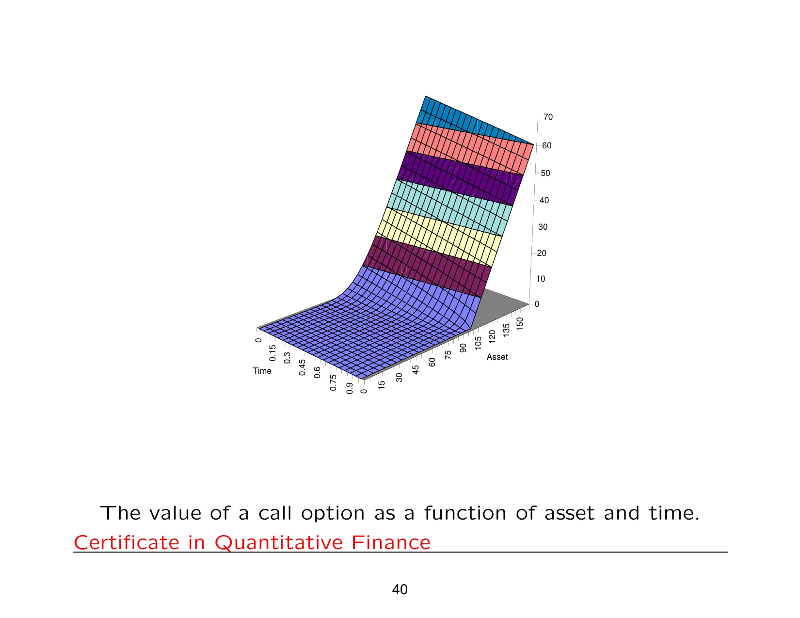
Because C is a function of two variables, it's a three-dimensional plot. This is what it looks like. If we were to take one slice, then we can go back here, some time prior to expiryexpiry The time at which an option or contract matures and its payoff is settled.. So this is C of S against S. That's what it looks like. So that's a two-dimensional cross-section.
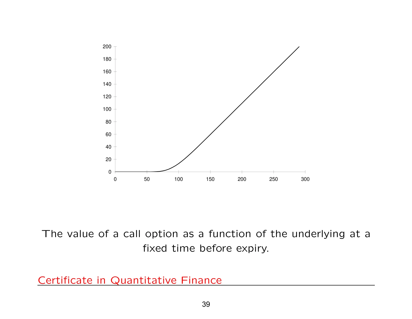
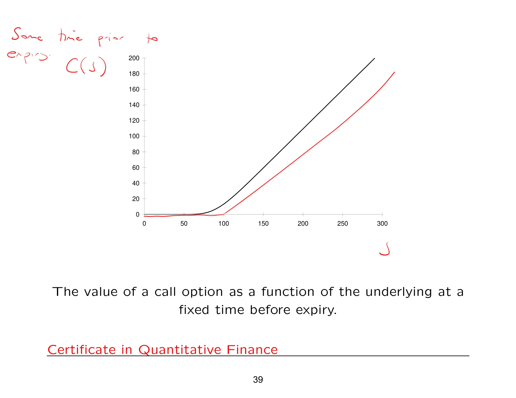
This is a two-dimensional plot. You've seen already what the payoff looks like. That's supposed to be a straight line, by the way. So the red line is the payoff, the black line is the price of the option some time prior to expiry.
There's the 3D plot. When there's a continuous dividend yieldcontinuous dividend yield / continuous and constant dividend yield D Continuous dividend yield is a dividend rate paid continuously rather than in discrete amounts., or there's also currency involved, this is what it looks like. Notice the previous formula looked like that, but now because of the continuous dividend yield, the impact is that our stock price is now being discounted by whatever the dividend yield is. So this is what it looks like in the presence of a continuous constant dividend yield. That's the extra term that's come in there.
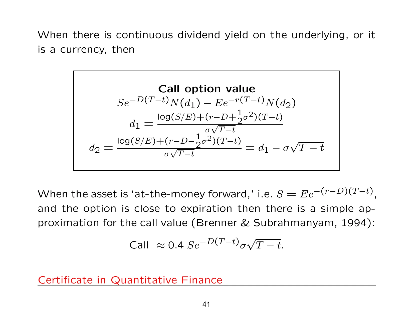
Now the next bit is something that's been, I know for a fact, asked at interviews. There's a class of options called at-the-money forward optionsat-the-money forward option An at-the-money forward option is an option whose strike equals the forward price of the underlying asset., which are struck when the strike price is equal to the forward priceforward price The price fixed today for delivery of an asset at a future date.. In other words, this.
You can easily, as an exercise, substitute this into here, wherever the E is, and then you get a closed-form solutionclosed-form solution A closed-form solution is an exact expression that can be written using standard mathematical functions and operations. for at-the-money forward optionsat-the-money forward option An at-the-money forward option is an option whose strike equals the forward price of the underlying asset.. In other words, ones that are simply struck at that particular point where E is equal to the forward priceforward price The price fixed today for delivery of an asset at a future date..
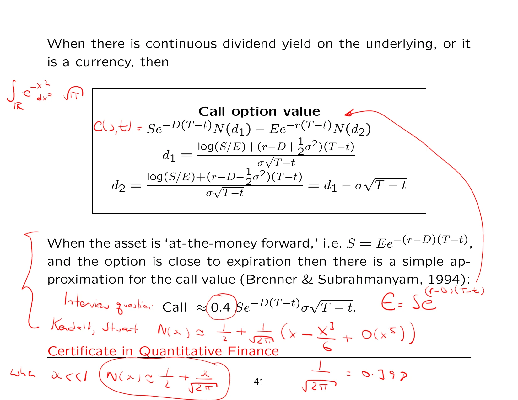
The reason why Paul's written down the next thing is because these two chaps came up with an approximation for at-the-money forward options when you're close to expiry. You can then use an approximation to N due to Kendall and Stewart.
So the first thing is simply to substitute the strike price into the formulas above, into d1, d2, and also C, then use this approximation by Kendall and Stewart. He said that N of x, I've written down as 1 over 2 plus 1 over root 2 pi, x minus x cubed over 6 plus x over 5. They come up with this.
When x is small, when x is very small, then N of x is, to leading order, just that term there. Sorry, there should be a 1 there. When x is very, very small, that's something you can easily try.
Simply substitute that value of E into that expression for C, and also d1 and d2.
Then just to leading order, it simply becomes that term there. Sorry, there should be a 1 there when x is very, very small. That's something you can easily try. Simply substitute that value of E into that expression for c, and also d1 and d2.
You'll then get a Black-Scholes pricing formulaBlack-Scholes pricing formula / Black-Scholes formulas The Black-Scholes pricing formula is the closed-form expression for the price of a standard option under the model assumptions. for an at-the-money forward option. And then if you replace the N with this approximation, also noting that 1 over root 2 pi is equal to 0.398, that's where the 0.4 comes from. So I've probably done most of the stuff for you. The only thing you need to do is some algebra, that's it. And you end up with that formula there.
I know a few people have been asked that question, to derive that approximation. Off the top of your heads, they expect you to know a lot more than just that. They expect you to know everything when you go for an interview. Most of the interviews are quite unreasonable anyway, but I thought I'd mention it. The other one I think I mentioned before was this one. That's also commonly asked.
arbitrage opportunities
Arbitrage is a pricing inconsistency that allows a profit without net risk in an idealized market.
Arbitrage is the possibility of making a profit from price differences for the same or equivalent asset, usually by combining trades that offset risk. In theory, an arbitrage-free market does not allow such a profit.
It is a core assumption in derivative pricing and is used to justify fair-value formulas. The absence of arbitrage is what makes the Black-Scholes framework mathematically meaningful.
The lecture uses arbitrage to motivate why the option price must satisfy a specific relationship with the underlying asset. The phrase appears when discussing what would happen if prices were inconsistent.
score: 16 · inline: first_in_lecture
At the money means an option’s strike price is equal, or nearly equal, to the underlying asset price.
At the money describes an option whose strike price is equal, or very close, to the current price of the underlying asset. It is one of the standard moneyness categories used for options.
Moneyness helps describe how an option’s payoff and value relate to the underlying price. It is a basic classification used throughout option pricing.
The lecture lists at the money alongside in the money and out of the money as part of the standard moneyness vocabulary. It serves as a reference point before moving to more specific pricing formulas.
score: 12 · inline: first_in_lecture
at-the-money forward options
An at-the-money forward option is an option whose strike equals the forward price of the underlying asset.
An at-the-money forward option is an option whose strike price is set equal to the forward price of the underlying asset. This definition uses the forward price rather than the current spot price.
Using the forward price can simplify pricing expressions and comparisons across maturities. It is a common setup in derivative pricing discussions.
The lecture mentions at-the-money forward options when deriving a Black-Scholes pricing formula. The term appears in the pricing setup rather than as a payoff category alone.
score: 17 · inline: first_in_lecture
The backward Kolmogorov equation is a PDE for the expected future value of a stochastic process, written backward in time.
The backward Kolmogorov equation is a partial differential equation that governs the evolution of expected future values of a stochastic process as time moves backward from a terminal condition. It is closely related to transition probabilities and conditional expectations.
It provides the mathematical bridge between stochastic processes and pricing equations. In option pricing, it helps explain why the value function satisfies a PDE.
The lecture identifies the pricing PDE as the backward Kolmogorov equation during the derivation. This connects the Black-Scholes equation to a standard result from stochastic calculus.
score: 16 · inline: first_in_lecture
Binary options are options with a payoff that takes one of two possible values, typically a fixed amount or zero.
Binary options are derivative contracts whose payoff has only two possible outcomes, such as paying a fixed amount if a condition is satisfied and nothing otherwise. They are also called digitals.
They are a simple example of a discontinuous payoff and are useful for understanding how payoff structure affects pricing. They also appear as building blocks in more complex derivatives.
The lecture introduces binary options while discussing payoff types and terminology. The alias digitals is mentioned as an alternative name in the same context.
score: 16 · inline: first_in_lecture
The binomial model is a discrete-time asset-pricing model with two possible moves at each step.
The binomial model is a discrete-time framework for modeling asset prices, where the price can move up or down over each time step. It is often used to build intuition for derivative pricing.
It provides a simple setting for replication, hedging, and no-arbitrage pricing. Many continuous-time results are motivated by taking a limit of the binomial model.
The lecture refers back to the binomial model as prior material and uses it as a comparison point for the Black-Scholes derivation. It helps motivate the continuous-time formulas.
score: 15 · inline: first_in_lecture
The Black-Scholes equation is the PDE that option prices satisfy under the Black-Scholes assumptions.
The Black-Scholes equation is a partial differential equation for the value of a derivative as a function of time and the underlying asset price. It arises from no-arbitrage arguments and hedging.
It is the central mathematical result behind the Black-Scholes pricing framework. Solving it leads to explicit pricing formulas for standard options.
The lecture presents the Black-Scholes equation as the main PDE obtained from the hedging argument. It is then used to derive pricing formulas and compare the result with the heat equation.
score: 18 · inline: first_in_lecture
The Black-Scholes model is a continuous-time framework for pricing options and other derivatives.
The Black-Scholes model is a continuous-time financial model that describes the evolution of an asset price and the pricing of derivatives written on it. It combines assumptions about the stock process, trading, and market frictions.
It is the foundation of modern option pricing and a standard reference point in quantitative finance. The model leads to the Black-Scholes equation and pricing formula.
The lecture introduces the Black-Scholes model as the main framework for the topic and says it consists of three key ingredients. Those ingredients are then used to derive the pricing equation.
score: 18 · inline: first_in_lecture
Black-Scholes pricing formula, Black-Scholes formulas
The Black-Scholes pricing formula is the closed-form expression for the price of a standard option under the model assumptions.
The Black-Scholes pricing formula is an explicit expression for the value of a standard option in terms of the underlying price, strike, time to maturity, volatility, interest rate, and related inputs. It is obtained by solving the Black-Scholes equation.
It gives a practical way to compute option prices without solving the PDE from scratch each time. It is one of the best-known results in derivative pricing.
The lecture uses the phrase when moving from the PDE to an explicit call and put price. The plural form appears when discussing formulas for both calls and puts.
score: 19 · inline: first_in_lecture
Boundary conditions are constraints imposed at the edges of a differential-equation problem.
Boundary conditions are extra constraints that specify the behavior of a solution at the boundaries of its domain. They are needed to determine a unique solution to many differential equations.
They are essential for solving PDEs and for turning a general equation into a specific pricing problem. In option pricing, boundary conditions encode payoff behavior at extreme asset prices or at maturity.
The lecture mentions a pair of boundary conditions while setting up the pricing PDE. They help determine the option value uniquely once the equation is established.
score: 12 · inline: first_in_lecture
A call option gives the holder the right, but not the obligation, to buy an asset at a fixed strike price.
A call option is a derivative contract whose payoff depends on the underlying asset price being above the strike price at expiration. Its value increases when the underlying price rises.
Call options are one of the basic building blocks of option pricing and hedging. They are the standard example used to explain payoff and pricing formulas.
The lecture writes down the call option payoff before deriving the pricing formula. It is used as the main example for the Black-Scholes calculation.
score: 12 · inline: first_in_lecture
The Cauchy-Euler equation is a type of differential equation with coefficients that scale with the variable.
The Cauchy-Euler equation is a differential equation whose coefficients are powers of the independent variable, often making it solvable by a power-law substitution. It is a standard form in differential equations.
It is useful as a comparison when transforming equations into more familiar forms. In this lecture, it helps illustrate the structure of the pricing PDE after a change of variables.
The lecture mentions the Cauchy-Euler equation while discussing how the transformed equation should be recognized. It serves as a mathematical comparison rather than the main result.
score: 11 · inline: first_in_lecture
closed-form solutions
A closed-form solution is an exact expression that can be written using standard mathematical functions and operations.
A closed-form solution is an explicit formula for a quantity, rather than a result obtained only through numerical approximation or iteration. It is usually expressed with standard functions and algebraic operations.
Closed-form solutions are valuable because they make analysis and computation simpler. In option pricing, they provide direct formulas for prices and sensitivities.
The lecture notes that the Black-Scholes derivation leads to a closed-form solution. This is presented as a major advantage of the model for pricing calls and puts.
score: 11 · inline: first_in_lecture
A constant coefficient partial differential equation is a PDE whose coefficients are constant rather than variable.
A constant coefficient partial differential equation is a PDE in which the coefficients multiplying the derivatives do not depend on the independent variables. Such equations are often easier to analyze than variable-coefficient PDEs.
Recognizing constant coefficients can simplify solution methods and transformations. In pricing theory, this helps connect the equation to standard forms like the heat equation.
The lecture describes the transformed pricing equation as a constant coefficient PDE. This observation supports the comparison with classical equations from mathematical physics.
score: 16 · inline: first_in_lecture
continuous dividend yield, continuous and constant dividend yield D
Continuous dividend yield is a dividend rate paid continuously rather than in discrete amounts.
Continuous dividend yield is a rate describing dividends as if they are paid continuously over time, typically as a proportion of the asset price. It is used as a simplifying assumption in pricing models.
Including dividend yield changes the drift and pricing formulas for the underlying asset. It is an important input when extending Black-Scholes pricing to dividend-paying stocks.
The lecture mentions continuous dividend yield when stating the model assumptions and adjusting the pricing setup. The notation in the source suggests a possible wording or transcription ambiguity.
score: 13 · inline: first_in_lecture
CDF stands for cumulative distribution function, the function that gives P(X ≤ x) for a random variable X.
CDF stands for cumulative distribution function. It is the function that assigns to each value x the probability that a random variable is less than or equal to x.
CDFs are standard tools for describing probability distributions and appear frequently in quantitative finance formulas. They help express option prices in terms of normal probabilities.
The lecture says the pricing expression can be written in terms of the cumulative distribution function. This is part of the step from the PDE solution to the final formula.
score: 13 · inline: first_in_lecture
d1, d2
d1 and d2 are the two standard intermediate quantities that appear in the Black-Scholes pricing formula.
d1 and d2 are notation for two intermediate expressions used in the Black-Scholes formula. They combine the underlying price, strike, time to maturity, volatility, and interest rate.
They are the arguments of the normal cumulative distribution functions in the final pricing formula. Understanding them helps interpret how the model inputs affect option value.
The lecture refers to d1 and d2 while discussing the final Black-Scholes expression and how people have tried to interpret them. They appear as part of the standard closed-form formula.
score: 19 · inline: acronym_only
Delta is the sensitivity of an option’s value to a small change in the underlying asset price.
Delta is a sensitivity measure that describes how much an option’s value changes when the underlying asset price changes by a small amount. In hedging, it is also the number of underlying units used to offset price risk.
It is one of the most important quantities in option risk management and replication. Delta links the derivative’s price movement to the underlying asset’s movement.
The lecture uses delta in the hedging argument and in expressions such as delta dS. It is treated as the hedge ratio that is kept fixed over a short time step in the derivation.
score: 13 · inline: first_in_lecture
delta-hedging
Delta hedging is a strategy that uses the underlying asset to offset changes in an option’s value.
Delta hedging is a hedging method in which the position in the underlying asset is adjusted so that the portfolio is locally insensitive to small price changes. The hedge ratio is given by delta.
It is the key idea behind the no-arbitrage derivation of the Black-Scholes equation. It shows how a derivative can be replicated by combining the option with the underlying asset.
The lecture presents delta hedging as the mechanism that removes risk over a short time step. It is used to motivate the differential equation for the option price.
score: 18 · inline: first_in_lecture
A portfolio constructed to offset price sensitivity to the underlying asset, at least for small moves.
A delta-hedged portfolio is a position whose exposure to small changes in the underlying asset price is offset by an opposite position in the underlying or related instruments. The goal is to make the portfolio’s value locally insensitive to price moves.
It is a standard way to manage risk in derivative pricing and hedging. It helps connect option values to the behavior of the underlying asset.
In this lecture, the term appears in the discussion of hedging as an example of how a trader can reduce risk by balancing exposures. It is part of the setup for understanding dynamic replication and option pricing.
score: 13 · inline: first_in_lecture
The process of valuing a derivative contract using a mathematical or financial model.
Derivative pricing is the task of finding the fair value of a contract whose payoff depends on another asset or variable. It usually relies on a model for the underlying asset’s dynamics and the contract’s payoff structure.
It is the central problem in much of quantitative finance. Understanding it explains how hedging, payoff structure, and market assumptions combine to produce a price.
The lecture uses this phrase to frame the topic and motivate the mathematical tools that follow. It signals that the discussion is about turning a payoff description into a pricing formula.
score: 10 · inline: first_in_lecture
An idealized distribution concentrated at a single point, used to model impulses and point sources.
The Dirac delta function is not an ordinary function but a distribution that is zero everywhere except at one point, where it is concentrated in an idealized way. It is used to represent point sources and to pick out values under integration.
It is a common tool in physics and PDEs for expressing localized inputs and initial conditions. In finance lectures, it often appears when discussing fundamental solutions and limiting behavior.
Here it is mentioned in connection with the limit as a time parameter becomes very small, where a solution behaves like a point source. That makes it useful for understanding the fundamental solution of the pricing equation.
score: 16 · inline: first_in_lecture
The strike price after discounting it back to present value.
The discounted strike price is the strike amount converted to present value using an appropriate discount factor. It represents the current-value equivalent of paying the strike at a future date.
Discounting is essential in option pricing because cash flows at different times are not directly comparable. It helps express a payoff in present-value terms.
The lecture uses this phrase when rewriting the option payoff in a form suitable for pricing and hedging arguments. It appears alongside the underlying asset price in the payoff expression.
score: 12 · inline: first_in_lecture
dividends on the underlying
Cash payments made by a company or asset to its holders, sometimes affecting option pricing.
Dividends are payments distributed to holders of an asset, most commonly shares of stock. In pricing models, they may be treated as discrete payments or as a continuous yield.
Dividends change the expected return and the forward-looking value of the underlying asset. They therefore affect derivative prices and hedging relationships.
The lecture contrasts cases with no dividends and cases where dividends are paid discretely on the underlying. This affects the setup of the pricing model and the payoff dynamics.
score: 13 · inline: first_in_lecture
The expected rate of change of a stochastic process over time.
The drift rate is the deterministic part of a stochastic process that describes its average tendency to increase or decrease. In a diffusion model, it is the coefficient of the term representing expected motion.
It is one of the basic parameters in models of asset prices and other random processes. It helps distinguish average trend from random fluctuation.
The lecture mentions the drift rate while discussing the assumptions behind the asset-price model. It is part of the parameter set used to describe the underlying process.
score: 12 · inline: first_in_lecture
A hedging method in which positions are updated repeatedly over time to maintain the desired risk exposure.
A dynamic hedging strategy is a hedging plan that is rebalanced over time rather than set once and left unchanged. It uses changing positions in the underlying or other instruments to keep the portfolio’s risk profile close to target.
Dynamic hedging is a core idea in derivative pricing because it links option values to replicating portfolios. It shows how risk can be managed through continuous or repeated adjustment.
The lecture presents hedging as an example of a dynamic strategy, emphasizing that the hedge is not static. This prepares the ground for the pricing argument based on repeated rebalancing.
score: 16 · inline: first_in_lecture
A payoff determined only at maturity, as in a European-style option.
A European payoff is a payoff that is realized only at the contract’s expiry date. It depends on the asset value at maturity rather than on any earlier exercise opportunity.
European-style payoffs are simpler to analyze than American-style payoffs because they remove early-exercise decisions. This makes them a standard starting point in option pricing.
The lecture identifies the payoff as European and equates it with a European call option. That helps narrow the pricing problem to a maturity-only payoff.
score: 13 · inline: first_in_lecture
The time at which an option or contract matures and its payoff is settled.
Expiry is the date or time when a derivative contract reaches maturity. After expiry, the contract’s payoff is determined according to its terms.
Expiry is a key feature of option contracts because the value depends on how much time remains. It also determines when the terminal payoff condition applies.
The lecture lists expiry as one of the contract features alongside strike. It is used when describing the payoff and the terminal condition at maturity.
score: 12 · inline: first_in_lecture
An equation that governs the time evolution of a process’s probability density.
The forward Kolmogorov equation describes how the probability distribution of a stochastic process changes over time. It is also known as the Fokker–Planck equation in many contexts.
It connects stochastic dynamics with PDE methods and is useful for deriving transition densities and fundamental solutions. In finance, it helps relate asset-price models to pricing equations.
The lecture identifies a PDE in the derivation as the forward Kolmogorov equation. This places the pricing discussion within the broader theory of diffusion processes.
score: 18 · inline: first_in_lecture
The price fixed today for delivery of an asset at a future date.
The forward price is the price agreed today for a transaction that will occur at a specified future date. It is determined by the current spot price, financing, and any income or carry effects in the model.
Forward prices are a basic benchmark in derivatives and arbitrage pricing. They help connect spot markets with future delivery contracts.
The lecture uses the forward price as the value that appears in the pricing relationship being derived. It serves as a reference point for the contract’s fair value.
score: 12 · inline: first_in_lecture
An idealized market in which trading can occur without costs or restrictions.
Frictionless markets are a modeling assumption in which assets can be traded continuously without transaction costs, taxes, bid-ask spreads, or other barriers. The assumption simplifies arbitrage and hedging arguments.
It makes mathematical pricing models tractable and allows clean replication arguments. Many core results in derivative pricing are derived under this idealization.
The lecture mentions frictionless markets when motivating the hedging setup and the ability to trade continuously. This assumption supports the derivation of the pricing equation.
score: 12 · inline: first_in_lecture
source solution
A solution of a PDE corresponding to a point source, often used as a building block for other solutions.
A fundamental solution is the response of a differential equation to a point source or impulse. More general solutions can often be built by combining or integrating these basic responses.
It is a central concept in PDE theory and helps explain how solutions propagate from localized initial data. In finance, it is useful for understanding pricing kernels and transition densities.
The lecture refers to the source solution or fundamental solution when discussing the PDE representation of the pricing problem. It is presented as the object that emerges from the short-time limit.
score: 21 · inline: first_in_lecture
A random process commonly used to model asset prices, with proportional changes and continuous randomness.
Geometric Brownian motion is a continuous-time stochastic process in which proportional changes in a variable follow a Brownian motion with drift. It is widely used to model stock prices because it keeps values positive.
It is one of the standard starting points for option pricing and risk-neutral valuation. Many classic results in quantitative finance are derived from this model.
The lecture states that the stock price satisfies a geometric Brownian motion, which sets up the later PDE and hedging arguments. It provides the stochastic dynamics for the underlying asset.
score: 18 · inline: first_in_lecture
Greeks, the Greeks
Sensitivity measures for an option or derivative with respect to key inputs.
The Greeks are quantities that measure how the value of an option or derivative changes when underlying variables change. Common examples include sensitivity to price, time, volatility, and interest rates.
They are essential for understanding and managing derivative risk. They also connect the pricing formula to practical hedging decisions.
The lecture repeatedly refers to the Greeks when discussing sensitivities and the meaning of the pricing equation. They appear as part of the interpretation of the model’s output.
score: 18 · inline: first_in_lecture
A function used to represent the response of a linear PDE to a point source or impulse.
A Green's function is a kernel that gives the solution of a linear differential equation produced by a point source. It can be used to construct solutions for more general inputs by integration.
It is a powerful tool for solving PDEs and understanding how local disturbances propagate. In pricing theory, it helps express solutions in integral form.
The lecture notes that the fundamental solution would be called a Green's function in this setting. This links the pricing PDE to standard methods for linear equations.
score: 16 · inline: first_in_lecture
heat equation, 1D heat equation, one-dimensional heat equation
The heat equation is a partial differential equation that models diffusion or heat flow in one spatial dimension.
The heat equation is a partial differential equation that describes how a quantity such as temperature changes over time as it spreads through space. In one dimension, it tracks diffusion along a line.
It is a standard model for diffusion processes and a useful mathematical analogue in option pricing. In this lecture, it helps connect the Black-Scholes derivation to a familiar PDE form.
The lecture refers to the 1D heat equation when comparing the pricing PDE to a classical diffusion equation. It is used as a reference point for recognizing the structure of the Black-Scholes equation.
score: 19 · inline: first_in_lecture
A diffusion-like partial differential equation with the same form as the heat equation.
A heat-type equation is a partial differential equation whose structure matches the classical heat equation or a closely related diffusion equation. It typically describes how a quantity spreads or smooths over time.
These equations are central in mathematical physics and quantitative finance because they are often solvable by standard PDE methods. They provide the framework for many pricing derivations.
The lecture says the pricing problem leads to a heat-type, or diffusion-type, equation. This identifies the mathematical form of the equation used to derive the option value.
score: 18 · inline: first_in_lecture
The act of reducing exposure to risk by offsetting a position with another position.
Hedging is the use of one or more positions to reduce the risk of losses from another position. In finance, it often means taking an offsetting position in the underlying asset or a derivative.
It is a core idea in risk management and derivative pricing. Hedging explains why certain portfolios are constructed and how sensitivities are controlled.
The lecture uses hedging to describe the risk-reduction goal behind the portfolio construction. It is part of the motivation for the dynamic strategy discussed in the example.
score: 14 · inline: first_in_lecture
An option state where exercising the contract would produce positive intrinsic value.
An option is in the money when exercising it would yield a positive payoff before considering any premium paid for the contract. The exact condition depends on whether the option is a call or a put.
It is a standard way to describe option moneyness and payoff status. It helps interpret whether a contract has intrinsic value at a given time.
The lecture uses the phrase when discussing the desired payoff outcome at expiry. It appears in the context of a European call option and its payoff region.
score: 11 · inline: first_in_lecture
Itô expansion, Itô 4
Itô expansion is the stochastic-calculus analogue of Taylor series for functions of processes driven by randomness.
Itô expansion is a formula that approximates the change in a function of a stochastic process, taking into account both ordinary differential terms and random fluctuations. In this lecture it is used in a specific version referred to as “Itô 4.”
It is a basic tool for deriving pricing equations when asset prices follow stochastic dynamics. It lets the lecture move from a random price process to a differential equation for the option value.
The lecture uses Itô expansion as the main calculus step in the derivation of the pricing PDE. The shorthand “Itô 4” refers to the particular version being applied here.
score: 21 · inline: first_in_lecture
Jump conditions specify how a variable must behave when a process changes abruptly.
Jump conditions are constraints imposed at a point where a model allows a sudden change or discontinuity. They describe the required relationship between values on either side of the jump.
They help make a model mathematically well defined when smooth evolution is interrupted by a jump. In pricing problems, they can determine how the value function behaves at special events.
The lecture mentions extra jump conditions as part of the derivation, indicating additional constraints beyond the main differential equation. They appear as technical conditions needed to complete the setup.
score: 12 · inline: first_in_lecture
log transformation, log of the price
A log transformation rewrites the price in logarithmic form so that changes are handled additively instead of multiplicatively.
A log transformation replaces a variable such as a price with its logarithm. This turns proportional changes into additive changes and often simplifies stochastic models.
It is useful in finance because asset prices often evolve multiplicatively, while logarithms make the algebra and calculus easier. It can also make distributions and differential equations more tractable.
The lecture uses a log transformation to work in terms of the log of the price rather than the price itself. This helps simplify the derivation of the pricing equation.
score: 14 · inline: first_in_lecture
no-arbitrage principle, no arbitrage
The no-arbitrage principle says that prices must not allow a riskless profit from a self-financing strategy.
The no-arbitrage principle is the assumption that a market should not permit a guaranteed profit without risk or net investment. It is a consistency condition on prices.
It is one of the main foundations of derivative pricing because it links the value of a contract to replication and discounting arguments. Without it, the pricing equation would not be pinned down in the same way.
The lecture invokes no-arbitrage to justify the relation between the derivative value and the risk-free growth rate. It is the key economic assumption behind the pricing derivation.
score: 22 · inline: first_in_lecture
The normal distribution is a symmetric bell-shaped distribution characterized by its mean and variance.
The normal distribution is a continuous probability distribution with a symmetric bell shape around its mean. It is fully determined by its center and spread.
It appears frequently in stochastic modeling because sums and transformations of random effects often lead to normal laws. Its cumulative distribution function is a standard tool for computing probabilities.
The lecture refers to the cumulative distribution function for the normal distribution when expressing the final pricing result. This connects the derivation to a standard probability function.
score: 12 · inline: first_in_lecture
The option price is the value at which an option is assumed or observed to trade.
The option price is the monetary value of an option contract at a particular time. In pricing theory, it is the quantity being solved for.
It is the central unknown in option valuation and the output of the pricing model. Understanding it is necessary for interpreting the final formula.
The lecture notes that one must agree on the option price before proceeding with the derivation. This makes the option price the target of the pricing argument.
score: 11 · inline: first_in_lecture
pricing of options
Option pricing is the task of determining the value of an option contract.
Option pricing is the mathematical and financial problem of assigning a value to an option contract. It uses assumptions about the underlying asset, time, and uncertainty.
It is a central topic in quantitative finance because option values depend on both market dynamics and contract terms. The lecture’s main goal is to derive a pricing formula from these assumptions.
The lecture frames the whole discussion as a breakthrough in option pricing and uses the term to introduce the pricing problem. The derivation then builds the option value from stochastic dynamics and no-arbitrage.
score: 21 · inline: first_in_lecture
Parabolic describes a class of partial differential equations with one time derivative and second-order derivatives in space.
Parabolic is a classification for certain partial differential equations, typically those with first-order time terms and second-order spatial terms. These equations often resemble diffusion or heat-flow models.
The classification helps identify the mathematical behavior of the equation and the methods used to solve it. In finance, it signals that the pricing equation has a diffusion-like structure.
The lecture explains that the pricing PDE is parabolic because it is first order in time and second order in the other variable. The term is used to classify the equation derived from the model.
score: 13 · inline: first_in_lecture
Path independent means the result depends only on the starting and ending points, not on the path taken between them.
A path-independent quantity has the same value regardless of the route used to get from one state to another. In calculus and finance, this often means the quantity can be written as a function of state variables only.
Path independence is important because it allows a model to be expressed as a well-defined function rather than a history-dependent process. That makes derivations and pricing formulas much simpler.
The lecture uses the phrase when discussing the structure of the pricing expression. It indicates that the value being derived does not depend on the specific path of the underlying process.
score: 12 · inline: first_in_lecture
A payoff is the amount received from a contract at maturity, usually as a function of the underlying asset price.
A payoff is the final value delivered by a financial contract when it expires. For options, it is typically a function of the underlying asset price at maturity.
The payoff is the starting point for pricing because the contract value today is derived from its future payment. Knowing the payoff determines what is being valued.
The lecture refers to the payoff repeatedly when setting up the option-pricing problem and when discussing the expected value to be discounted. It is the future quantity whose present value is being computed.
score: 15 · inline: first_in_lecture
PDE, partial differential equation, partial differential equations, PDEs
PDE stands for partial differential equation, an equation that relates an unknown function to its partial derivatives.
A PDE is an equation involving an unknown function of several variables and its partial derivatives. It describes how the function changes with respect to more than one independent variable.
PDEs are the standard mathematical language for many continuous models in physics and finance. In option pricing, the value of the derivative is often characterized by a PDE.
The lecture repeatedly refers to deriving and solving the PDE for the option price. Here, the PDE is the main equation produced by the no-arbitrage argument.
score: 25 · inline: acronym_only
PDF, probability density function
PDF stands for probability density function, the function that describes the density of probability for a continuous random variable.
A PDF is a function used for continuous random variables to describe how probability is distributed across values. Probabilities over intervals are obtained by integrating the density.
It is a standard tool for computing expectations and probabilities in continuous models. In pricing, it helps express expected values in integral form.
The lecture uses PDF when discussing multiplication by a density and when identifying a distributional form. It appears in the step where an expectation is written using a continuous probability density.
score: 15 · inline: acronym_only
Present value is the value today of a future cash flow after discounting.
Present value is the amount that a future payment is worth at the current time after applying a discount factor. It converts future money into today’s terms.
It is a core concept in valuation because pricing compares future payoffs with current prices. Discounting is what links expected future outcomes to a present market value.
The lecture describes the option price as the present value of an unknown function and later as the present value of a function W. This reflects the discounting step in the pricing derivation.
score: 17 · inline: first_in_lecture
The present value of the expected payoff is the discounted current value of the payoff averaged over its probability distribution.
This phrase refers to taking the expected future payoff and discounting it back to the present. It combines probability weighting with time-value-of-money adjustment.
It captures the basic logic of many pricing formulas: estimate the future payoff, average over uncertainty, then discount to today. This is a central idea in derivative valuation.
The lecture uses this phrase as the pricing target after applying no-arbitrage and probability arguments. It summarizes the final valuation idea in the derivation.
score: 20 · inline: first_in_lecture
A put option is a contract whose payoff increases when the underlying asset price falls below the strike price.
A put option is a derivative contract that gives a payoff based on the right to sell an underlying asset at a specified strike price. Its value depends on the asset price relative to that strike.
Put options are a standard example in option pricing and are often used to illustrate valuation formulas. They provide a concrete payoff structure for the lecture’s derivation.
The lecture explicitly writes down a put option as part of the pricing setup. It serves as the example contract for the formulas being developed.
score: 12 · inline: first_in_lecture
Put-call parity is the relationship between the prices of a put and a call with the same strike and expiration.
Put-call parity is an identity that links the prices of a put option and a call option with the same strike and maturity. It reflects the fact that certain combinations of contracts have the same payoff.
It is a fundamental consistency relation in option pricing and helps connect different derivative prices. It also supports valuation arguments based on replication and no-arbitrage.
The lecture mentions put-call parity as part of the derivation strategy. It is used to relate the put option being discussed to other pricing expressions.
score: 16 · inline: first_in_lecture
Real-world drift is the expected rate of change of an asset price under the actual probability model.
Real-world drift is the drift parameter in a stochastic model under the real-world probability measure. It represents the average directional tendency of the asset price in that model.
It distinguishes the actual modeled growth rate from the rate used for pricing under no-arbitrage arguments. This distinction is important in stochastic finance.
The lecture names the real-world drift as mu when setting up the asset-price dynamics. It contrasts with the risk-free rate used later in the pricing argument.
score: 12 · inline: first_in_lecture
A risk-free portfolio is a portfolio whose value is designed to be free of uncertainty over a short time interval.
A risk-free portfolio is a portfolio constructed so that its value has no exposure to the modeled risk over the period of interest. In theory, its return is tied to the risk-free rate.
It is a key idea in replication arguments and no-arbitrage pricing. By comparing a derivative position with a risk-free portfolio, one can derive a valuation equation.
The lecture asks whether there is another risk-free portfolio, using the phrase in the context of constructing a hedged position. This supports the no-arbitrage derivation.
score: 15 · inline: first_in_lecture
risk-free rate, risk-free interest rate
The risk-free rate is the benchmark interest rate used for discounting and comparison in pricing models.
The risk-free rate is the return associated with a benchmark investment assumed to have no default risk. In models, it is often denoted by r.
It is the discount rate used in many valuation formulas and the reference return in no-arbitrage arguments. It anchors the pricing of derivatives and other claims.
The lecture introduces the risk-free interest rate and later writes the pricing relation using r. It is the rate that replaces the real-world drift in the no-arbitrage setup.
score: 18 · inline: first_in_lecture
Scalar multiplication means multiplying an object by a scalar, or ordinary number.
Scalar multiplication is the operation of multiplying a quantity by a single number rather than by another vector or matrix. It scales the size of the quantity without changing its basic form.
It appears throughout algebra, calculus, and finance when positions or terms are scaled by coefficients. In derivations, it helps combine and compare quantities with different weights.
The lecture uses the phrase when manipulating terms in the pricing derivation. It refers to scaling one quantity by a numerical factor.
score: 8 · inline: first_in_lecture
short the share
Short selling is a trading strategy where an investor sells an asset they have borrowed, hoping to repurchase it later at a lower price.
Short selling means taking a position that profits if the asset price falls. The seller borrows the asset, sells it, and later buys it back to return it.
It is a standard market mechanism used in pricing and hedging discussions, especially when analyzing payoffs and portfolio positions. In this lecture, it helps explain how the underlying share can be treated in the model.
The lecture uses short selling as part of the setup for the portfolio and assumes it is allowed for the underlying share. The phrase "short the share" is used as a shorthand for this position.
score: 17 · inline: first_in_lecture
sigma squared
Sigma is a parameter in the model, typically representing volatility or a volatility-related quantity.
Sigma is a symbol used for a model parameter, often the volatility of the underlying asset or a quantity derived from it. In formulas, sigma squared means the square of that parameter.
It controls the size of random fluctuations in the model and therefore affects pricing and risk calculations. Understanding sigma is essential for following the lecture's equations.
The lecture treats sigma as one of the constants in the model alongside other parameters such as the drift or interest rate. It appears in terms like sigma squared and in expressions involving the stock price.
score: 14 · inline: first_in_lecture
Similarity reduction is a method for simplifying a problem by using a change of variables that exploits its scaling structure.
Similarity reduction is a mathematical technique that transforms a problem into a simpler form by combining variables into a reduced set. It is often used when the equations have a scaling pattern or repeated structure.
It can turn a difficult partial differential equation or differential equation into one that is easier to solve. In quantitative finance, it helps derive closed-form expressions from model equations.
The lecture mentions similarity reduction as part of the method used to solve the pricing problem. It is presented together with substitutions and transformations as a way to simplify the equation.
score: 13 · inline: first_in_lecture
Stochastic calculus is the calculus of random processes, used to model and manipulate quantities that evolve with uncertainty.
Stochastic calculus extends ordinary calculus to processes with randomness, such as Brownian motion and diffusion models. It provides tools for differentiating and integrating random time-dependent quantities.
It is the mathematical framework behind many asset-pricing and risk models. Without it, the lecture's equations for the value process cannot be derived or interpreted properly.
The lecture introduces stochastic calculus as the mathematical setting for the model and then applies it to the value process dV. It is the background needed for the later derivation.
score: 16 · inline: first_in_lecture
strike price, strike
The strike price is the contract price used to exercise an option, also called the strike.
The strike price is the predetermined price written into an option contract. It is the level at which the holder may buy or sell the underlying when the option is exercised.
It is one of the main contract terms that determines an option's payoff and value. Comparing strike price with the forward price is part of the lecture's pricing discussion.
The lecture refers to strike as one of the key contract features, alongside expiry. It also states a case where the strike price equals the forward price.
score: 19 · inline: first_in_lecture
Substitutions and transformations are algebraic or variable changes used to simplify a problem before solving it.
These are methods that replace variables or rewrite expressions so a difficult equation becomes easier to handle. They often work by converting the original problem into a standard form.
They are common tools for solving differential equations and pricing equations in quantitative finance. They help reveal structure that is not obvious in the original variables.
The lecture mentions using substitutions and transformations as part of the solution method. They appear alongside similarity reduction in the derivation.
score: 9 · inline: first_in_lecture
terminal condition, final condition
A boundary condition specified at the final time, often equal to the option payoff at expiry.
A terminal condition is the condition imposed at the end of the time interval in a time-dependent equation. In option pricing, it is typically the payoff at expiry.
It anchors the solution of the pricing equation and allows the value at earlier times to be determined. Without it, the problem is not fully specified.
The lecture uses the terminal condition to mean the payoff at expiry and then works backward to earlier times. It also refers to final conditions in the same sense.
score: 15 · inline: first_in_lecture
Time to expiry is the amount of time remaining until a contract or option expires.
Time to expiry measures how long is left before the contract reaches its expiration date. It is usually treated as a variable in pricing formulas.
It affects the value of options and other derivatives because the remaining time changes the chance of different outcomes. Many pricing equations are written in terms of time to expiry.
The lecture rewrites the solution in terms of time to expiry and uses it as the main time variable. This helps express the pricing result in a standard form.
score: 14 · inline: first_in_lecture
Transaction costs are the expenses associated with buying or selling an asset.
Transaction costs are the costs that arise when a trade is made. They include explicit fees and other frictions that make trading more expensive than the quoted price.
They affect whether a trading strategy can be implemented exactly and can change theoretical pricing arguments. In finance models, they are often assumed away to simplify the analysis.
The lecture states that there are no transaction costs on the underlying, which is part of the model assumptions. This simplifies the derivation of the pricing result.
score: 10 · inline: first_in_lecture
transition density for a stock price, transition density function, transition density function for a stock price, transition PDF
A transition density is the probability density of the future value of a process given its current state.
The transition density describes how likely a stochastic process is to move from one value to another over a specified time interval. For a stock price, it gives the density of the future price conditional on the current price.
It is a core object in stochastic modeling because it summarizes the process's probabilistic evolution. In pricing, it helps connect the dynamics of the stock price to the distribution used in calculations.
The lecture refers to the transition density function for a stock price and uses it as part of the solution discussion. It is also mentioned in shorthand as the transition PDF.
score: 20 · inline: first_in_lecture
The underlying is the asset or instrument on which a derivative contract is written.
The underlying is the reference asset whose price determines the value of a derivative. In options, it is typically the stock, index, commodity, or other traded asset being modeled.
Derivative payoffs and pricing formulas are defined in relation to the underlying asset. Understanding which asset is underlying is essential for interpreting the contract and the model.
The lecture uses the underlying as the asset in the pricing setup and notes an assumption about its dividends. This keeps the focus on the stock-price dynamics.
score: 9 · inline: first_in_lecture
volatility of the stock
Volatility is a measure of the size of price fluctuations in an asset or model.
Volatility describes how variable an asset's price is over time. In quantitative finance it is often represented as a parameter in the model.
It is one of the main inputs in pricing and risk calculations because larger volatility usually means greater uncertainty. Many formulas in the lecture depend on volatility directly.
The lecture treats volatility as a key parameter that participants may agree on, and later refers to the volatility of the stock. It appears in the equations alongside other constants.
score: 17 · inline: first_in_lecture